
6. Advanced Functions
6.1 Calibration of Tool Center Point (TCP)
Calibrating the tool coordinates TCP is a crucial step to ensure precise positioning of the EWAS robot welding torch. Users can follow the steps below for calibration:
6.1.1 Calibration preparation
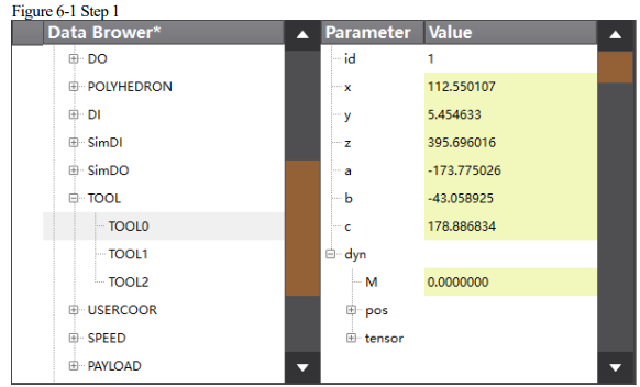
Step 1: Prepare a calibration cone with the pointed end facing upward, positioned on the worktable. Enter the program data interface and select the tool coordinates you want to calibrate, such as TOOL0, as shown in the figure below.
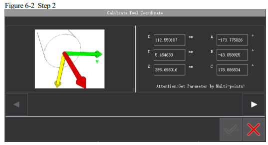
Step 2: Click "Modify", and you will enter the preview interface for the reference coordinate system, as shown in the figure below.
Step 3: Click "Settings" to enter the calibration method selection interface for the reference coordinate system, as shown in the figure below
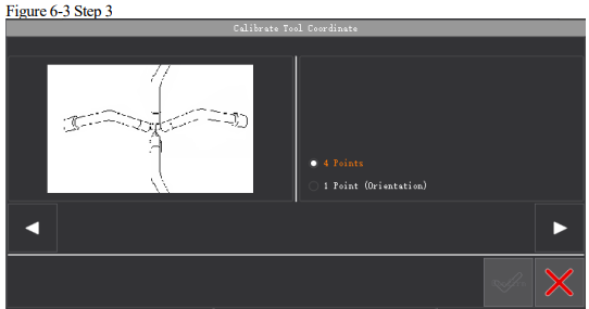
Step 4: Choose the calibration method for offset or posture.
6.1.2 4-point Calibration
Select the “4-point Calibration”, which means that you need to calibrate tool offset by teaching 4 different postures of the same point. Click "Next". Move the robot TCP to a position and click "Teach", as shown in figure below.
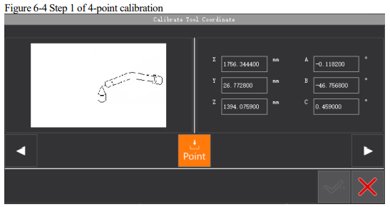
Then, click "Next" to change the posture of the robot, and click "Teach", as shown in figure below.
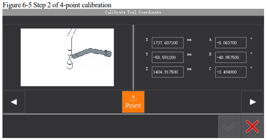
Click "Next" to change the posture of the robot, and click "Teach", as shown in figure below.
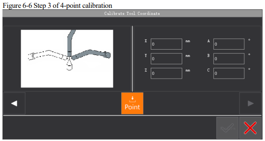
Click "Next" to change the posture of the robot, and click "Teach", as shown in figure below.
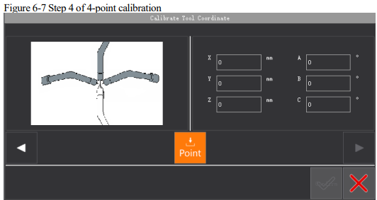
The accuracy error after this teaching will appear. User can continue to save the result or recalibrate as needed.
Click "Next" to get the calibrated value, as shown in figure below.
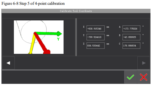
Click "OK" after it is confirmed to be correct. The modification is finished.
6.1.3 One-point Calibration
Select "One-point Calibration" to indicate the posture of the next calibration tool. It can only
calibrate the posture change if a tool in an axis direction under tool coordinates. Click "Next".
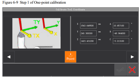
Make the direction of the robot's end in parallel to the Z axis, and click "Teach", as shown in figure below.
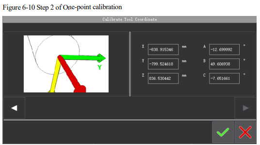
Click "Next", and the result of the posture calibration of tool coordinates will appear, as shown in figure below.
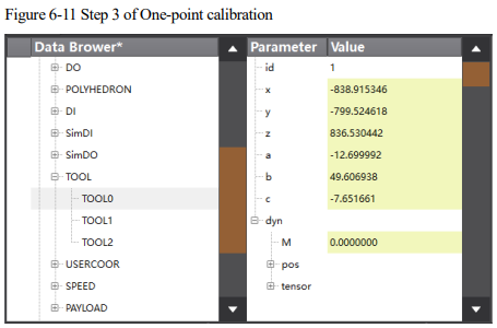
Click "OK" after it is confirmed to be correct. The modification is finished, as shown in figure below.
6.2 External Axis Coordination
When using external axis coordination for the first time, you can access the welding settings interface from the main screen of the teach pendant. Click on the "Advanced Settings" button for external axis coordination in the bottom navigation bar, or press the Fn+F2 key combination to bring up the external axis coordination interface, as shown in the figure below.
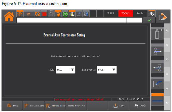
Select the appropriate tool as the current tool and choose the suitable positioner coordinate system as the reference coordinates. Click the "Save" button to save your current selections.
The next time you use this function, press the External Axis Coordination key  on the teach pendant once. At this point, the green indicator light in the upper left corner of the button will illuminate. The current tool and current reference coordinates on the teach pendant interface's upper right corner will switch to the results you saved during your last use. The current JOG coordinate system will become the positioner coordinate system.
When you want to stop using this function, press the External Axis Coordination key once again.
The green indicator light will turn off, and the above status indicators will return to their default settings.
6.3Additional Axis Encryption
This function is developed to facilitate the adaptation of ESTUN's additional axis for users. Users will need to provide the corresponding machine code to the vendor. To use this function, go to
Welding Application→ Advanced Settings→ Additional Axis Encryption, or press the key combination Fn+F3 in the Welding Application →Advanced Settings screen to bring up the following screen interface:
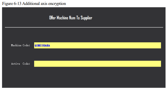
The machine code is generated by the system automatically. Users can send the machine code to our technical personnel. After our technical personnel provide the activation code, you can validate whether the machine code and activation code match by clicking the OK button. This is to ensure that the added additional axis is a product from our company.
6.4Hardware Testing
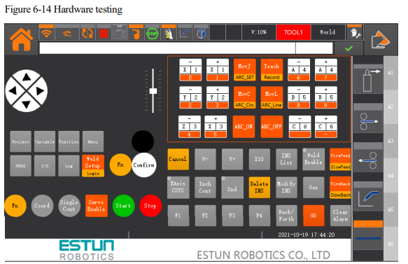
The hardware testing function is designed to allow users to test if each physical button on the teach pendant is functioning properly. To enable this function, you can access the hardware settings interface by clicking on "Advanced Settings" and then "Hardware Settings", as shown in the figure below. By pressing the corresponding buttons, the corresponding indicators in the interface will turn re.
6.5 Conveyor Tracking
6.5.1 Function overview
The conveyor tracking is designed to synchronize the movement of the robot and the workpieces on a conveyor, which move along the conveyor as it runs. The position information of the workpiece is obtained through a visual system or sensor, and transmitted to the robot via a designated interaction method. This allows the robot to pick up the workpiece from a fixed or moving conveyor based on the feedback from the sensor. There are two types of conveyors available, namely linear and disc-shaped.
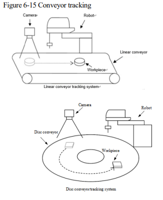

To access the conveyor configuration interface, users can click on "User Application-Conveyor Tracking" in the teach pendant. In this interface, conveyor parameters can be configured, including enabling the conveyor belt, checking and calibrating the pulse equivalent, viewing the conveyor belt position and speed, and toggling the display of reasons for non-tracking. Users can also switch between five configuration pages, namely "Conveyor Parameters", "Tracking Parameters", "Trigger Parameters", "Visual Parameters", and "Virtual Conveyor Belt", to further configure the settings.
6.5.2 Configuration of conveyor parameters
Select [Conveyor Parameters] and choose either [Linear Type] or [Disc Type] in the "Type" column. This will allow you to enter the configuration interface for both linear conveyors and disc conveyors respectively.
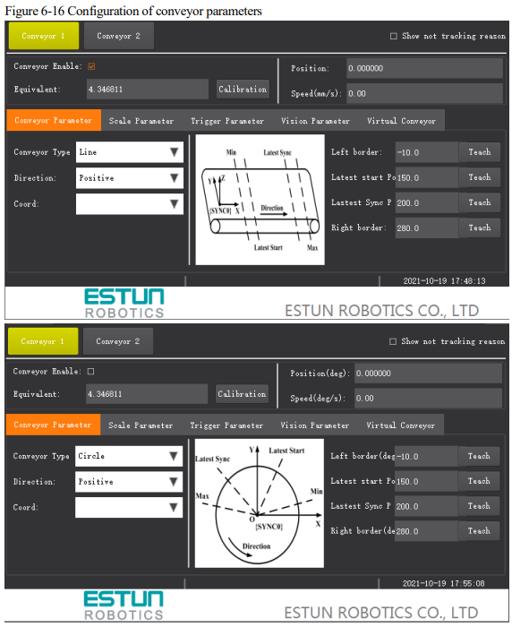
⚫ Type: linear or disc.
⚫ Direction: set the direction of the conveyor.
⚫ Moving coordinate system: The moving coordinate system bound to such conveyor.
⚫ Min./max. boundary/latest start point/latest synchronization point: For a linear conveyor, these represent the coordinate values in the X-direction in the corresponding moving coordinates. For a disc conveyor, they represent the angle at the center of the XOY plane in the corresponding moving coordinates.
6.5.3 Tracking parameters configuration
Select "Tracking Parameters" to enter the conveyor parameters configuration interface.
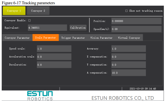
⚫ Velocity coefficient/Accel coefficient/Decel coefficient: the ratios of the velocity/Accel/Decel during the tracking synchronization process.
⚫ Tracking tolerance: the threshold used to judge the accuracy of the tracking synchronization, representing the maximum allowable displacement error between the robot and the target object.
⚫ X-axis compensation: the compensation for workpiece offset relative to the target position in the X direction.
⚫ Y-axis compensation: the compensation for workpiece offset relative to the target position in the Y direction.
⚫ A-axis compensation: the compensation for workpiece offset relative to the target position in the A direction.
6.5.4 Trigger parameter configuration
Select "Trigger Parameters" to enter the trigger parameter configuration interface.
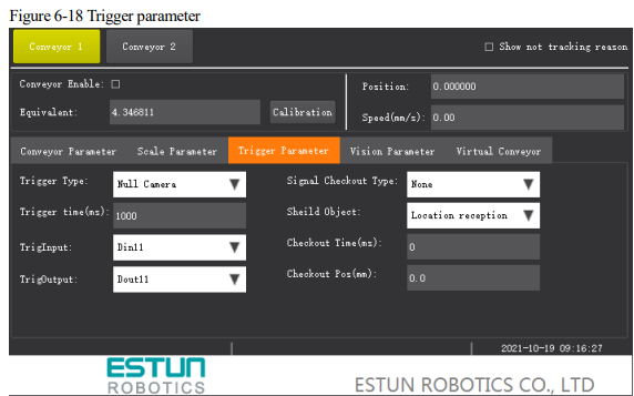
⚫ Trigger Types:
Timing trigger: The system will output a high level signal from the trigger output port based on the configured trigger time (ms) and cycle, of which high-level hold time is 1/2 of the trigger time.
External IO trigger: When the system detects a rising edge signal at the trigger input port (detection cycle of 4ms), set the trigger output port to output a high level signal. The high-level hold time is synchronized with the trigger input port.
Non-camera trigger: No visual operation mode, and a task program needs to be created: detecting input signals, sending target information, and so on. RUN program can be used to write the commands. When the rising edge signal is detected at the trigger input port, call the SetTargetPos to send the workpiece position information.
⚫ Trigger time: The settings are valid when the "Trigger Type" is of "Timed Trigger". It indicates the interval time for inputting the high level signal at the specified trigger output port.
⚫ Trigger input port: Specify the trigger input port information for system detection. The settings can be valid when the "Trigger Type" is of "External IO Trigger" or "Non-Camera Trigger".
⚫ Trigger output port: Specify the trigger output port information output by the system, so that the camera can perform shooting. The settings can be valid when "Trigger Type" is of "Timed Trigger" or "External IO Trigger".
6.5.5 Visual parameter configuration
Select [Visual Parameters] to enter the visual parameter configuration interface.
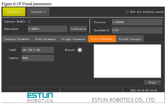
⚫ Visual IP: Set to the IP address of the camera.
⚫ Port Number: The default port number is 5500.
⚫ Connection Status: Display the connection status with the camera server. GREEN indicates a connected status, GREY indicates a disconnected status, and Colorless indicates an unconnected status.
6.6Multi-station Reservation
6.6.1 Function overview
With this function, the robot can complete tasks on up to 4 stations without intermittent.
Multi-station Reservation function works to bind each station in the robot working area to different input ports, and assign these input ports with the functions of starting and stopping, and then the user can enable the robot to execute the station program bound to it automatically by entering effective signal to the input port. Also, by using this function, user can start the programs on the corresponding tooling in turn according to the sending order of the signals.
The figure below illustrates a working example of a robot: its working sequence is tool 1, tool 2 and tool 3; the jobs performed on each tool are program 1, program 2 and program 3.
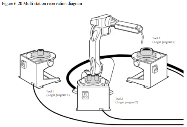
Each of the three toolings process the different workpieces, corresponding to different processing procedures. There’re following two effects when starting it under Playback mode, assuming that the procedures are program 1, program 2, and program 3:
⚫ When there’s no program executed currently, user sends signal to tool 1, and the robot will automatically load and run program 1. The starting mode of tools 2 and 3 is the same as the tool 1.
⚫ The program currently being executed by the robot: Assuming that program 1 is currently being executed, and workpieces are prepared for tools 2 and 3, the user first sends the starting signal to tool 3, and then the tool 2. At this moment, as the robot is executing the tool 1, then the system will record the appointment waiting status of tools 3 and 2 in turn. When program 1 is executed, the robot will execute program 3 first, and then the program 2. The whole appointment process is finished by this moment.
When the robot operates, the user can check the working status and IO signal of each station using the teach pendant.
6.6.2 Way of use
To use this function correctly, user needs to complete the following tasks:
⚫ The program of each station has been edited correctly. For the editing method of the program, please refer to the Programming Commands.
⚫ The Start button located on the tooling of each station can be used properly.
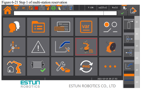
Step 1 Click "Multi-station Reservation" in the "User Application" plug-ins on the Home interface, as shown in the two figures below.
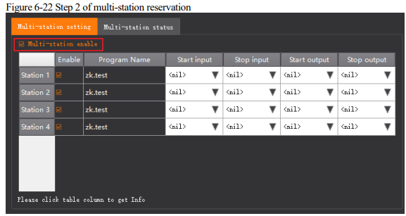
Step 2 After entering "Multi-station Reservation Settings", check "Multi-station Reservation Enable" and the "station" to be operated.
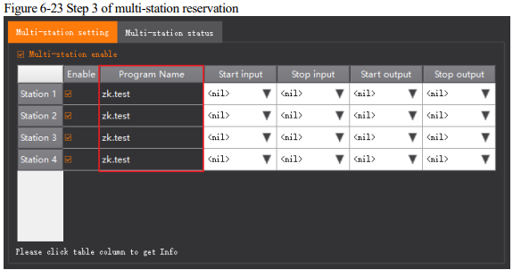
Step 3 Click the "program name" in the row where each "station" is located.
Step 4 Select the program you want to perform from the "Project List".
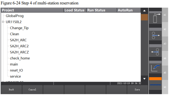
⚫ Click "Back" to return to the "Multi-station Reservation Setting" interface.
⚫ Click "Clear" to reset the "Preset Program" of the "Station".
⚫ Click "Select" to preset the currently selected "Program" to this "Station", and return to the "Multi station Reservation Setting" interface.
Step 5 Assign the "Start Input", "Stop Input", "Status Output" and "Stop Output" signals to each "station" correctly.
Note: Repeated use of the unified IO ports is not allowed.
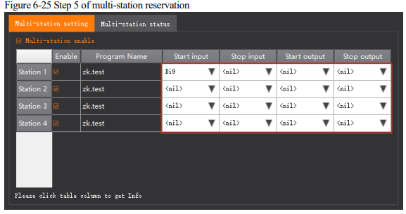
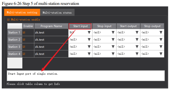
Users can click each cell in the table header listed on the interface to view the “Help” information.
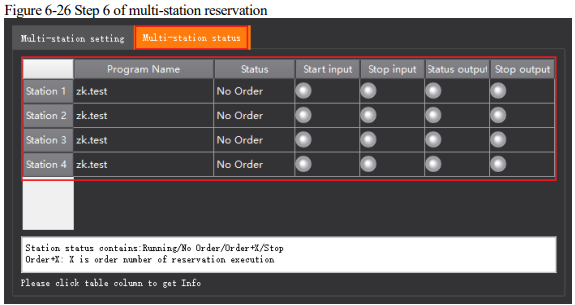
Step 6 Click "Multi-station Reservation Status" to view the status of each "Station" as well as its IO signal status.
[Note]
⚫ After the parameters of the Multi-station Reservation are properly set, you can perform the multi-station reservation operation after switching the system to Playback mode.
When a program is not executed and the reservation is successfully made, but you then want to cancel the current reservation, just cancel the reservation by inputting signal to the start unit.
6.7 Maintenance
6.7.1 Function overview
This function is primarily used to remind users to perform timely maintenance and service on the robot to prevent a reduction in its lifespan due to prolonged use without maintenance.
There are two ways in which reminders are provided during usage:
⚫ Accumulated running time: Each model corresponds to a maintenance execution cycle (e.g. 10,000 hours, 11,520 hours, etc.). When the maintenance execution time exceeds this cycle, the system will prompt "Maintenance overdue, please maintain in a timely manner!".
⚫ Use date: Each model corresponds to a cumulative usage period (e.g. 2 years, 3 years, etc.). From the factory/execution date to the end of the usage period, which is the next maintenance date, the system will prompt "Maintenance overdue, please maintain in a timely manner!".
6.7.2 Way of use
Step 1: On the Home interface, click on "Maintenance Tips" within the "User Applications" plugin group, as shown in the figure below.
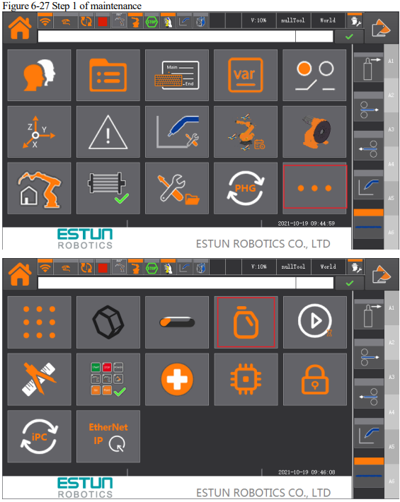
Step 2 Enter the "Maintenance Tips" interface, as shown in the figure below:
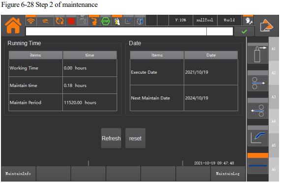
Step 3: Interface introduction:
⚫ Total running time: The accumulated running time of the robot since the factory, this value keeps accumulating and cannot be cleared.
⚫ Maintenance execution time: The running time accumulated since the factory or reset
⚫ Maintenance execution cycle: Each model has a corresponding maintenance cycle (e.g. 10,000 hours, 11,520 hours, etc.). When the maintenance execution time exceeds the maintenance execution cycle, the maintenance tips will appear.
⚫ Manufacture/execution date: The date when the robot's control system first runs or when it is reset.
⚫ Next maintenance date: The date of the next maintenance. When the system date is later than the next maintenance date, the maintenance tips will appear.
Step 4: Operation introduction:
⚫ Refresh: Click "Refresh" to get the current maintenance information again.
⚫ Reset: Click "Reset" and enter the dynamic password to execute. There is special software to get the dynamic password through verification code. Please contact relevant technical personnel to obtain the dynamic password.
Resetting will clear the "Maintenance Execution Time" and set the "Manufacture/Execution Date" and "Next maintenance date" to the current system date.
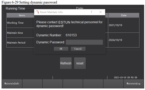
Step 5: Prompt information:
⚫ Prompt Log: The information of recent maintenance tips will be saved, as shown in figure below. Click "Prompt Log" to access historical prompt records.
⚫ Prompt contents: If the maintenance cycle or date has passed, a reminder with code 53006 will be displayed.
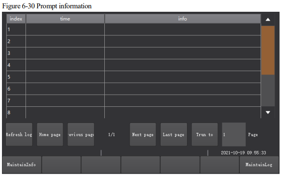
[Note]
⚫ After the due date or maintenance cycle, please perform maintenance promptly. If not maintained in a timely manner, the prompt information will appear during normal use of the robot.
6.8Multi-type Area Monitoring
6.8.1 Function overview
By setting up safety zones, the position of the robot can be monitored in real time under a variety of working conditions, minimizing the likelihood of collisions.
Multi-type area monitoring consists of the following three main types:
⚫ WorkArea:
All CheckPoints (TCPs) of the robot are only allowed to move within the WorkArea. In the event of a violation of the WorkArea rules, there are two ways of handling:
When the robot leaves the WorkArea, the program stops and alarms.
When the robot enters the WorkArea, it continues its operation and outputs a signal.
⚫ BlockedArea
All CheckPoints (TCPs) of the robot are not allowed to move within the BlockedArea. In the event of a violation of the BlockedArea rule, there are two ways of handling:
When the robot leaves the BlockedArea, the program stops and alarms.
When the robot enters the BlockedArea, it continues its operation and outputs a signal.
⚫ SignalArea
All CheckPoints (TCPs) of the robot are only allowed to move within any areas. In the event of a violation of the WorkArea rules, there are two ways of handling:
When the robot enters the signal work area, it continues to run the program and outputs a signal
When the robot leaves the signal work area, it continues to run the program and outputs a signal
6.8.2 How to use standard area monitoring
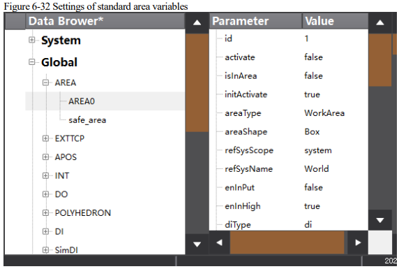
Step 1 Go to the program data interface and click on the standard area variable you want to set in the global domain, e.g. AREA0.
Step 2 Click on "Modify" and you will be taken to the interface for setting the area variable. By default, the standard area variable is "inactive" and the user can activate it by clicking "Activate".
Step 3 Click on "Modify" as shown in the figure below.
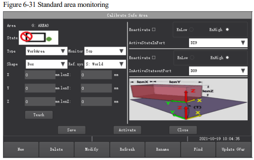
Step 4 Modify the parameters of this interface as described below.
⚫ Area Name: Display the name of standard area variable
⚫ Status: Determine if the TCP point is inside or outside the area when the area is active.
⚫ Type: Select the type of the area:
⚫ Reference Coordinates: Select the reference coordinates for this area, which defaults to the World Coordinates.
⚫ Shape: Choose the shape of the area, currently supporting BOX and CYLINDER shapes.
⚫ Input Ports: Check "Port Enable" to select the input ports that activate variables within this area. Specify whether they are "Low Active" or "High Active".
⚫ Output Ports: Check "Port Enable" to select the output ports that activate variables within this area. Specify whether they are "Low Active" or "High Active".
⚫ X, Y, Z, lenX, lenY, lenZ: Set the starting coordinates and size of the area. The starting coordinates are relative to the reference coordinates.
Step 5 Click "OK" to complete the setting of the standard area variables, as shown in figure below
[Note]
1. When the standard area is in an active state and the area type is either WorkArea or BlockedArea, the system will periodically check the robot's TCP point position during operation, providing real-time output regarding whether the robot is within the defined area.
2. When the standard area is in an active state and the area type is a signal area, the system wil periodically check the robot's TCP point position regardless of whether it is powered up. It will continuously provide real-time output regarding whether the robot is within the defined area.
3. After enabling the output ports, signals can be generated based on the robot's presence within the defined area.
4. After enabling the input ports, you can activate or freeze the area using a rising edge trigger on the DI (coexisting with standard area activation commands, standard area freeze commands, and whichever is triggered later).
5. When the "activate" parameter in the AREA-type variable is set to true, it defaults to automatically activating this standard area. The system will reevaluate this upon loading the AREA-type variable. If the DI port is not enabled, the area automatically activates. If the DI port is enabled, the area's activation is determined by the state of the DI signal.
6. The activation or freezing of standard areas can be executed through the variable configuration interface, commands, or input ports (as configured).
6.8.3 Method for using Polyhedron area monitoring
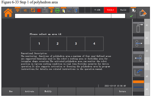
Step 1: When using the "Polyhedron Area" monitoring function, the polyhedron area needs to be configured first.
Click on "User Application > Polyhedron Area" to enter the Polyhedron Area plugin interface, as shown in figure below. Currently, up to 4 polyhedron regions are supported;
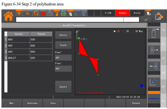
Step 2: Select the Area ID that you wish to configure. For instance, if you choose Area ID "1", you will enter the configuration interface for that area, as shown in the figure below. If this polygonal area has not been configured yet, you will receive a prompt stating, "This area does not exist; please create it!" In this case, click the "Create" button to enter the configuration interface.
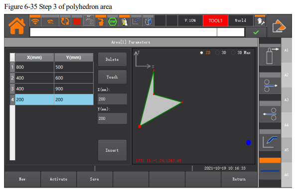
Step 3: Modify the parameters of the interface according to the following instructions:
⚫ Status: After activation of this area, determine whether the TCP point is inside or outside the area.
⚫ Auto Activation: When selected, this area will be automatically activated after the controller starts.
⚫ Type: Select the type of this area.
⚫ Coordinate System: Select the reference coordinates for this area, which defaults to the World Coordinates.
⚫ Vertex Z Value: Indicate the starting position of the area in the Z-direction of the coordinates. It can be entered manually or obtained by clicking the "Get Current Z Value" button. The result is obtained by subtracting the vertex height value from the Z-axis coordinate in the current coordinates.
⚫ Area Height: Indicate the height of the area in the Z-direction of the coordinates. It can be entered manually or calculated by clicking the "Calculate Z-Height" button, which displays the Z-axis coordinate value of the current coordinates minus the vertex height value.
⚫ Count of Vertices: Indicate the count of vertices on the bottom of the polyhedron area. Clicking on "Vertex Information" will bring up the vertex configuration interface, as shown in Figure 7-2. Clicking on "Add" will automatically add the current TCP position in the user coordinates. If you need to modify a vertex of the polyhedron area, select the corresponding vertex and modify it by clicking on "Teach" or entering the XY coordinates. If you need to delete a vertex of the polyhedron area, select the corresponding vertex and click on "Delete". The right side of the interface supports the preview of the 2D and 3D effects of the polyhedron area, as well as the enlarged 3D effect of only the polyhedron area. Preview supports synchronous display of the monitoring point position (blue dot in the figure). In 2D mode, only the position of the TCP point in the XY plane is displayed, and switching to 3D mode can preview the relative position of the actual TCP point;
⚫ Input Port: Check "Port Enable" to select the input port that needs to activate this area variable, and set it to "Low Active" or "High Active".
⚫ Output Port: Check "Port Enable" to select the output port that needs to activate this area variable, and set it to "Low Active" or "High Active".
Step 4: Click "Save" after completing the settings.
Step 5: When using a polyhedron area in the command, create a POLYHEDRON type variable and specify the correct polyhedron area ID in the "index" parameter. After creation, activate or deactivate the polyhedron area using the PolyhedronAreaActivate or PolyhedronAreaDeactivate command.
1. When the polyhedron area is activated and the area type is a WorkArea or a BlockedArea, the system will periodically check the TCP point position during operation and output the robot's status in the set area in real time.
2. When the standard area is activated and the area type is a signal area, the system will periodically check the robot TCP point position regardless of whether the excitation is on or off and output the robot's status in the set area in real time.
3. After setting the automatic activation parameter for the polyhedron area, it will not take effect immediately. The system will load the polyhedron parameters during a restart and determine whether to activate the area automatically based on the DI port status. When the DI port is disabled, the area is automatically activated, and when the DI port is enabled, the area is activated or not depending on the DI level.
4. The logic for activating or deactivating the polyhedron area is the same as the usage status of the input/output port and standard area monitoring function.
5. The activation or deactivation of the polyhedron area can be performed through the variable configuration interface, commands, or input ports (if configured).
6.9Collision Detection
6.9.1 Function overview
The collision detection function can detect whether the robot collides in real-time without the need for an external force sensor. If a collision is detected, the robot will immediately alarm and stop working, providing safety protection and effectively reducing the damage to the robot or other equipment. Users can turn ON or OFF the collision detection function according to the needs of the site. For safety reasons, it is recommended to turn on the collision detection function.
6.9.2 Way of use
To access the collision detection settings, select the "Common Settings" group on the System Home, and click on "Collision Detection," as shown in the figure below.
[Note]
If the current robot model does not support collision detection functionality, the interface will display "Collision detection is not supported by this model".
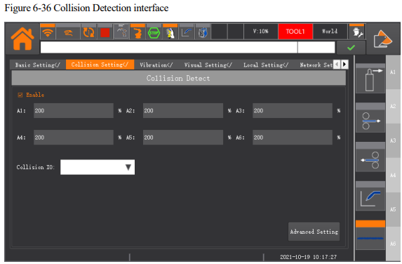
⚫ Enable: Checking this option enables collision detection, while unchecking it disables collision detection.
⚫ A1 to A6: These settings determine the sensitivity of collision detection, with a default value of 100.
A higher value results in lower sensitivity, whereas a lower value increases sensitivity in collision detection.
[Note]
⚫ This function detects collisions based on load information and device information, so the load information must be set correctly to avoid false alarms or affect detection sensitivity. For setting the load parameters, please refer to "PAYLOAD0" and "SetPayload" commands.
⚫ Different working conditions and operating conditions may result in different collision sensitivities with the same parameter settings. Therefore, false alarms may occur. If a collision false alarm occurs, appropriately reduce the sensitivity of the collision axis according to the alarm information by increasing the numerical value until the false alarm no longer occurs.
6.10 Vibration Suppression
6.10.1 Function overview
The Vibration Suppression function is used to reduce residual vibration at the end of the robot, allowing for smoother motion, to improve positioning accuracy, and shorter positioning time. The strength of the residual vibration varies depending on the robot's movement path, as well as its speed and end load. Typically, high-speed movement and heavy end loads are more likely to cause vibration and produce stronger vibrations.
6.10.2 Way of use
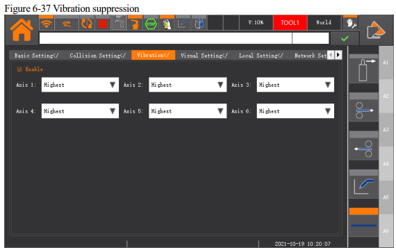
Select the "Common Settings" group on the System Home and click on "Vibration Suppression", to enter the configuration interface as shown in the figure below.
Users can tailor the vibration suppression settings to different application scenarios and requirements. By checking the "Enable" checkbox in the vibration suppression interface, users can then set the "Intensity" level for vibration suppression. There are five intensity levels available for vibration suppression: Low, Low-Medium, Standard, Medium-High, and High. The vibration suppression effect progressively strengthens with each higher intensity level. The default setting is the Standard intensity level.
[Note]
When using the Vibration Suppression function, it is essential to set the correct payload parameters, which affect the controller's adjustment of vibration suppression. Refer to the Basic Setting Interface for Setting Payload Parameters and the SetPayload Command for information on setting payload parameters.
6.11System IP Setup
6.11.1 Network settings
System IP Setup is only available to users with "Administrator" user type.
Select "Advanced Settings" on the System Home and click on "Network Settings" to enter the system "Network Settings" page. The teach pendant will display the corresponding setting page according to the controller system version.
To ensure normal communication, the parameters in this interface should be set to the correct values according to the actual situation.
Network Settings A
The controller system uses internal bridging for its network card. When any network port is connected to a LAN, the IP addresses of the teach pendant, OS1, and OS2 cannot be the same as those of other devices on the LAN, otherwise network address conflicts may result in communication anomalies.
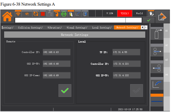
⚫ Remote Network Settings: Modify the IP addresses of the OS ends that are currently connected to the programming pendant remotely.
OS1 IP: IP address of OS1.
OS2 IP-TP: IP address of OS2.
OS2 IP-Comm: IP address used for communication with OS2.
⚫ Local Network Settings: Only modify the IP addresses of the OS ends that are locally connected to the programming pendant.
Programming pendant IP: IP address of the programming pendant.
OS1 IP: IP address of OS1.
OS2 IP-TP: IP address of OS2.
Network Settings B
The controller system divides the network into internal and external networks. The internal network is mainly for the effective connection between the programming pendant and the controller, while the external network is for the effective connection with external communication.
Therefore, when wiring the robot group, only ETH1 or ETH2 needs to be modified according to the application.
[Caution]
External communication network addresses cannot be the same as the identification segment of the internal communication network, otherwise normal communication may be affected. (For example, the default factory network segment for the internal network is 192.168.6.x, so the external network is not allowed to be set to 192.168.6.x.)
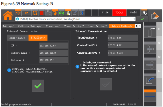
⚫ External Communication Network Settings:
ETH1(lan3): controller-side lan3 port, supports TCP/IP, ModbusTCP, etc.
ETH2(lan4): controller-side lan4 port, supports VNC, EtherNet/IP, Script, etc.
⚫ Internal Communication Network Settings: (default settings cannot be modified, please contact the manufacturer if necessary)
TeachPendant: IP address of the programming pendant.
ControllerOS: IP address of the controller.
ContollerRTOS: IP address of the controller's real-time system.
6.11.2 IP Scan
⚫ When the controller system is set to type B in the network settings, this function is temporarily unavailable.
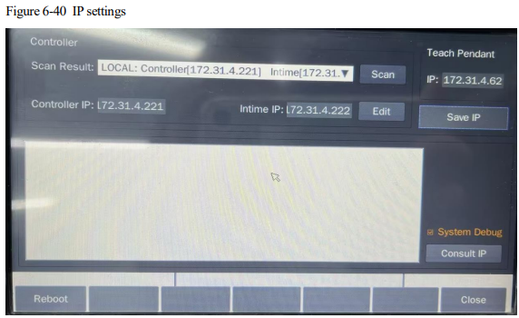
⚫ In some customer sites, there may be multiple controllers on the same LAN. Without clearing the controller IP configuration, the programming pendant may not be able to connect to the correct controller. Therefore, this function enables scanning of all controllers' IPs on the LAN using the teach pendant, allowing the customer to choose which controller to connect to.
⚫ If the teach pendant is unable to connect to the controller after starting up, you can access the IP configuration interface by pressing the following combination shortcut keys: Fn + "Welding Settings/Login" + "Logs" + "Position" + "I/O" + "Variables".
⚫ In the IP configuration interface, the IP can be directly edited, or the "Scan" button can be clicked to automatically search for the IP of the current LAN controllers and their corresponding real-time system IPs.
Selecting from the drop-down list will automatically fill in the configuration field.
⚫ After clicking "Save IP" and successfully saving the changes, click "Restart". After the restart, the programming pendant will be connected to the specified controller.
6.12 Upgrade and Backup of Teach Pendant
6.12.1 Program upgrading
Following two upgrading methods are available:
⚫ ESTOOL operation
Upgrade the program directly to the programming pendant system, without checking the "Upgrade the teach pendant while starting up". Load the program in the teach pendant system directly when it is powered on.
⚫ Upgrading plug-ins through TP
To upgrade the program of the pendant to the controller system, check the "Upgrade the teach pendant whil starting up", and load the program in the controller system directly when it is powered on. When this method is selected, the controller system version will be upgraded, and the pendant will also be upgraded automatically and synchronously.
Settings of update mode
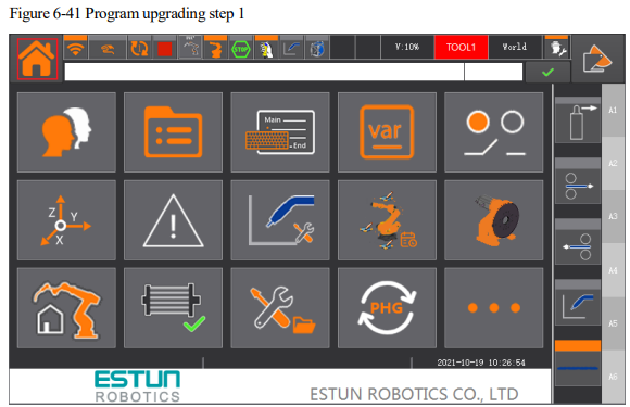
Step 1 Switch the user to the “Administrator”, and click the Advanced Settings plug-in group, as shown in figure below.
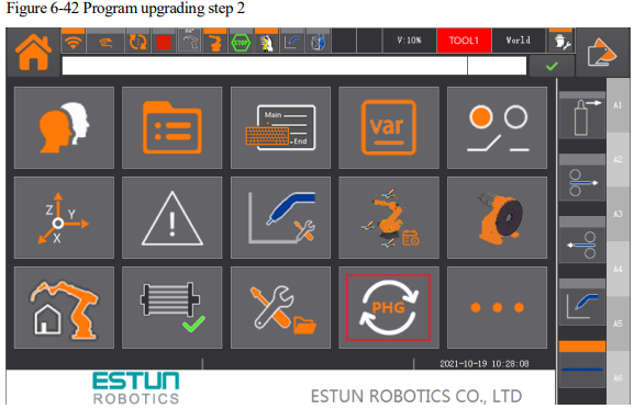
Step 2 Upgrade plug-ins in TP mode, as shown in figure below.
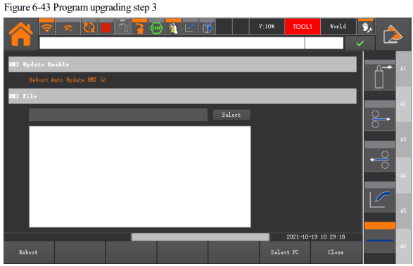
Step 3 Enter the TP update interface, and check the "Upgrade the teach pendant while starting up" to enable the synchronous update of the teach pendant.
ESTool update
Step 1 Start ESTool.
Step 2 ESTool login interface is shown in figure below
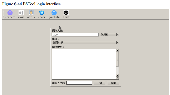
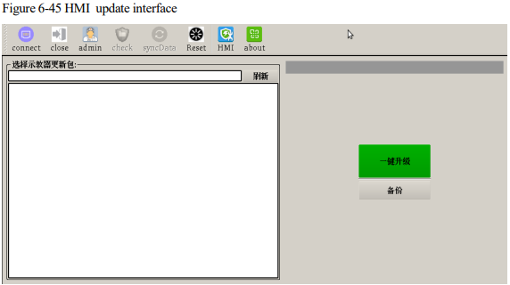
Step 3 HMI update interface after login, as shown in figure below. Select HMI function module, insert USB flash drive into the teach pendant, select the file to be updated on the left, and click the update button to update.
Update plug-ins for HMI
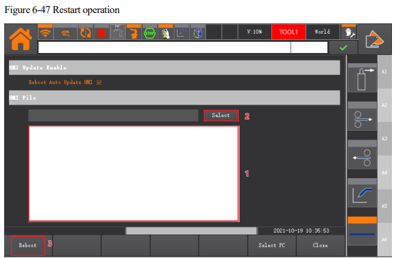
Step 1 Switch the user to the “Administrator”, and enter the TP update plug-ins in the Advanced Settings, as shown in the figure below.
Step 2 Select the pendant program file that needs to be updated in the USB flash drive from the list of pendant programs, and click "Select".
Step 3 A prompt message will pop up after the update is finished, as shown in the figure below.
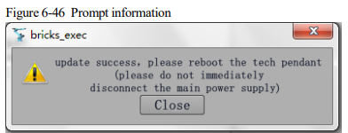
Step 4 Click "Restart", the teach pendant will restart and upgrade to the latest TP version automatically.
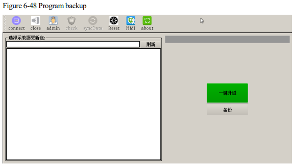
6.12.2 Program backup
Click the Backup button in figure below to export the current teach pendant program to the USB flash drive.
6.13 Update of Controller Operating Programs
6.13.1 Update of controller programs
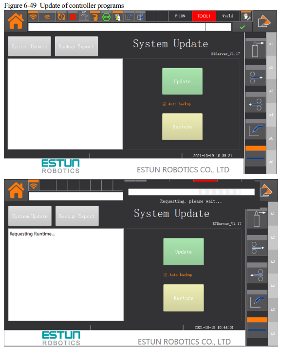
To update the controller running program, you need to follow the procedures below.
Step 1: Put the controller runtime program (.runtime or .patch format file, which is usually provided by the developer) into the root directory of the USB flash drive.
Step 2: Insert the USB flash drive into the Programming pendant USB port, select Advanced Settings on the System Home and click on the controller update interface as shown in figure below.
Step 3: Check the "Auto backup in the background" function if required; if checked, the existing system software will be backed up on the controller side before the update, and the backed up system software will be used to restore the system during the system restore.
Step 4: Click on the [Update] button, enter the administrator password to confirm and then you will be prompted if you need to export the existing runtime. Select "Yes" to export the existing runtime from the controller, and select
"No" to skip this step and continue to the next step.
Step 5: After selecting the update file, it will automatically update, then wait for the completion of the update.
[Note]
⚫ When updating the controller, and "Auto background backup" is checked, then a backup of the runtime process will appear during the update, as shown in the figure below;
⚫ If the actual programming pendant is used and updated from a USB flash drive, then the USB flash drive must be in FAT32 format;
⚫ Whether it's a USB flash drive update or a direct update using the virtual teach pendant, the name of the update package and the path where it is located must not contain Chinese characters;
⚫ Do not power down your system while the system update is in progress, in case the system update is not completed and the system does not function properly.
6.13.2 Controller program restoration
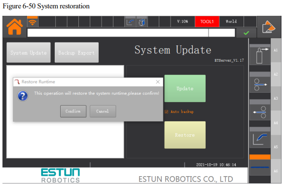
The following steps are used for restoring the controller program:|
Step 1: Switch to Administrator mode, access the controller upgrade interface, and click "Restore". to enter the administrator password for confirmation. After that, a confirmation dialog box will pop up.
Step 2: Once the controller approves the restoration request, the restoration operation will begin.
Step 3: Wait patiently for some time. The teach pendant will display a message box indicating that the restoration is about to end. To ensure data synchronization, the teach pendant needs to be restarted. For the virtual teach pendant, automatic restart is not possible, so after clicking "OK", the virtual teach pendant will close automatically, and you need to manually reopen and run it. For the physical teach pendant, it will restart automatically after you click "OK".
[Note]
Do not turn off the system power while waiting for the system restoration to complete to avoid system malfunction caused by the restoration failure.
6.13.3 Backup export
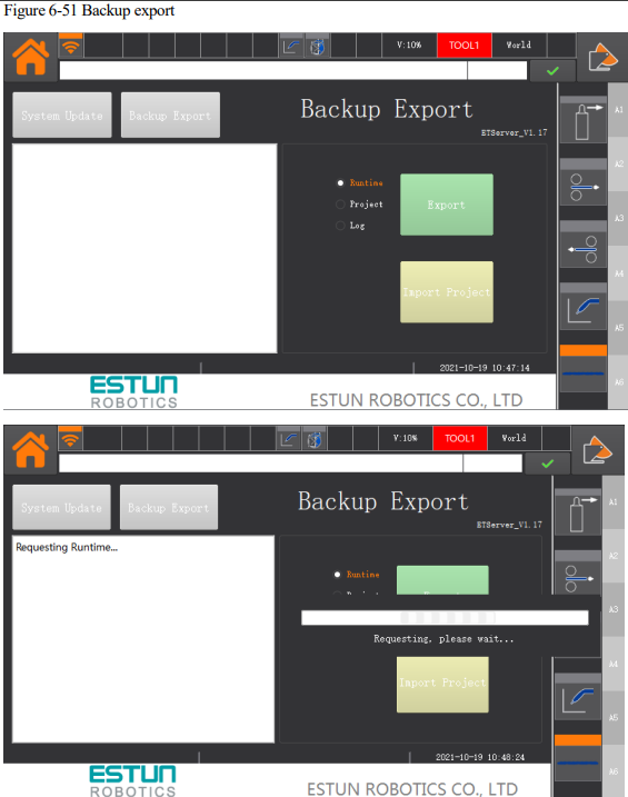
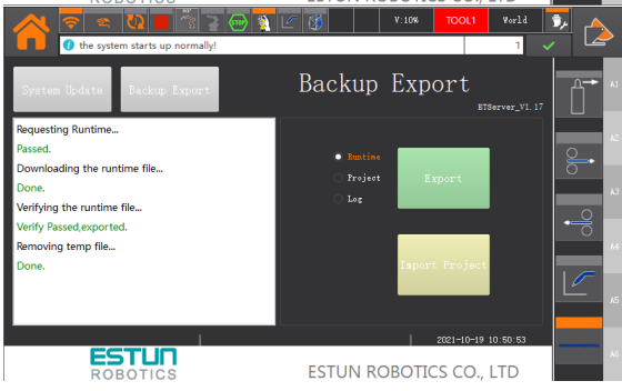
Step 1: Switch to administrator mode, access the "Controller Upgrade" interface, click "Backup Export", and display the backup export interface as shown in figure below.
Step 2: Select the export type as required (including: runtime package, project program, and system log), then click "Export". Enter the administrator password for confirmation (if the actual programming pendant is used and no Udisk is inserted, a prompt to insert the U-disk will appear), and then request export to the controller, as shown in figure below.
Step 3: After the request is approved, the "Export Rename" dialog box will appear. The virtual Programming Pendant also supports selecting the directory to save the export. After setting the export name, click "OK" to begin exporting the corresponding file.
Step 4: After the export is complete, it will be displayed as shown in figure below.
[Note]
If using the physical teach pendant, do not remove the U flash drive before the export is complete, as it may cause the exported files to be nonexistent or damaged;
6.13.4 Project import
Step 1: Put the prepared project file (.project format file, which can be obtained by using the backup export function to export the project program. If it needs to be made under special circumstances, = please refer to the Operation Manual for ER Series Industrial Robot Controller Upgrade) into the root directory of the USB flash drive and insert the USB flash drive into the programming pendant.
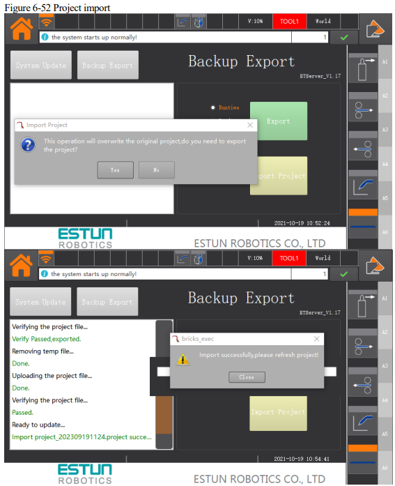
Step 2: Switch to the administrator user and enter the "Controller Upgrade" interface. Click "Backup Export" and then click "Import Project". After entering the administrator password to confirm, the interface shown in figure below will be displayed, prompting that importing the project will overwrite the existing project. You can choose to export the existing project by clicking "Yes". The process is the same as exporting the project program. After the export is completed, the project program file dialog box will be entered. If you click "No", you will directly enter the dialog box for selecting the project program file.
Step 3: Select the imported project program, and the import will begin. After the import is completed, the prompt "Import successful" will be displayed. Please refresh the project, as shown in figure below.
Step 4: Click the project button on the right to enter the project interface. Click "Refresh" to display the imported project.
6.14 Reach by One-Click
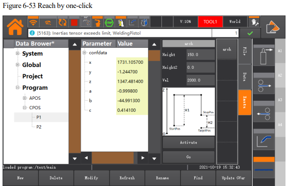
Reach by one-click. With this function, the robot moves from the current point to the target point in an arched path. The user interface is shown in figure below.
[Note]
⚫ This function is currently available only on SCARA models.
⚫ Reach by one-click. It is applicable only to position variables in the world coordinates.
⚫ When being activated, the parameter configuration of Reach by One-click will become valid.
⚫ To use this function, press and hold the hand switch in manual mode before performing motion operations.
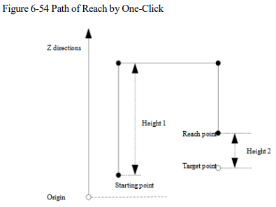
⚫ By pressing and holding the button, the robot will stop after moving to the target point. If the button is released halfway, the robot will stop motion immediately, and continue to move toward the target point by pressing such button again. Where: Height 1 represents the height of the vertical lift from the starting point along the z-axis;
Height 2 represents the vertical height of the target point. The arched path is shown in figure below.
6.15 Laser Welding Calibration
6.15.1 Calibration steps
The calibration involves establishing the conversion relationship between the laser coordinates and the robot coordinates, enabling the conversion of weld seam positions detected by the laser into robot coordinates, which are then communicated to the robot.
Preparations and considerations before calibration are as follows:
1. The robot must have undergone calibration to ensure accuracy and correctness of the tool and robot coordinates.
2. The laser must be securely and correctly mounted according to the laser's operational instructions.
3. Personnel performing the calibration should wear protective eyewear and avoid prolonged direct exposure to the laser.
4. Throughout the calibration process, the robot should be switched to the tool coordinate system. Conditions for Laser Calibration:
1) The robot must have undergone calibration to ensure accuracy and correctness of the tool and robot coordinates.
2) The laser must be securely and correctly mounted according to the laser's operational instructions.
3) Personnel performing the calibration should wear protective eyewear and avoid prolonged direct exposure to the laser.
4) TCP calibration (as illustrated with TOOL0 in the diagram below) should be performed first, followed by laser calibration.
Click  in the laser calibration interface to enter the interface, as shown in figure below.
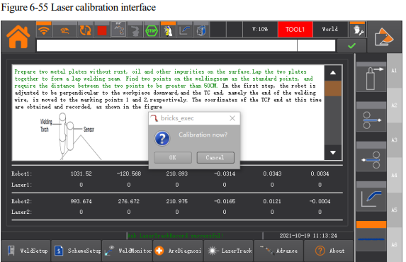
Click "OK" to proceed with the laser calibration or click "Cancel" to abort the calibration. You can review the points and calibration matrix recorded from the previous calibration.
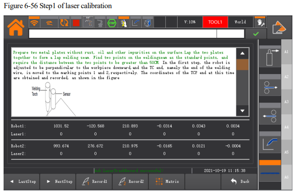
Prepare two metal plates with surfaces free of rust, oil, or impurities. Overlap these two plates to create a lap joint, forming a weld seam. Select two points on this weld seam as calibration points, and make sure that the two points are at least 30CM apart. Before starting the calibration, ensure that the laser is turned on, which requires executing the "ConnectLaser" command in the
program.
Step 1: Adjust the robot's posture to be vertical above the workpiece and move the TCP end effector to calibration points 1 and 2. Record the coordinates of the robot's TCP end effector at these positions, as shown in the diagram.
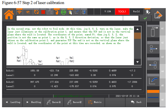
Step 2: Set the robot to Tool mode. In this mode, you can jog the robot's TCP in the X, Y, and Z directions to turn on the laser and position it to shine directly onto calibration point 1. Ensure that the TCP end effector is not in the same vertical plane as the weld seam. Record the coordinates of this point and name it as "P1"; next, jog the TCP in the X, Y, and Z directions to make sure it is not in the same position as point 1. If there’s deviation in the X, Y, or Z direction, position the laser to shine directly onto calibration point 2. Again, ensure that the TCP end effector is not in the same vertical plane as the weld seam. Record the coordinates of this point and name it as "P2," as shown in the figure below.
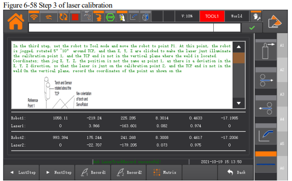
Step 3: Set the robot to Tool mode and move it to point P1. In this position, jog the robot to rotate around the TCP by 5° to 10°. Then, jog the robot in the X, Y, and Z directions until the laser is shining directly onto calibration point 1. Ensure that the TCP end effector is not in the same vertical plane as the weld seam, and record the coordinates of this point. Next, jog the robot in the X, Y, and Z directions, making sure it is not in the same position as point 1. If there’s deviation in the X, Y, or Z direction, position the laser to allow it to emit directly onto calibration point 2. Again, ensure that the TCP end effector is not in the same vertical plane as the weld seam.
Record the coordinates of this point, as shown in the figure below.
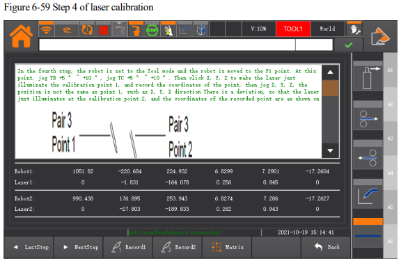
Step 4: Set the robot to Tool mode and move it to point P1. In this position, jog TB by +5° to +10° and TC by +5° to +10°. Then, jog the robot in the X, Y, and Z directions until the laser is emitting directly onto calibration point 1.
Record the coordinates of this point. Next, jog the robot in the X, Y, and Z directions, to ensure that it is not in the same position as point 1. If there’s deviation in the X, Y, or Z direction, position the laser allow it to emit directly onto calibration point 2. Record the coordinates of this point, as shown in the figure below.
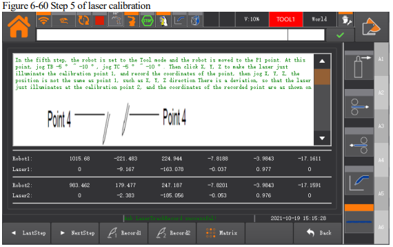
Step 5: Set the robot to Tool mode and move it to point P1. In this position, jog TB by -5° to -10° and TC by -5° to - 10°. Then, jog the robot in the X, Y, and Z directions until the laser is emitting directly onto calibration point 1.
Record the coordinates of this point. Next, jog the robot in the X, Y, and Z directions, to ensure that it is not in the same position as point 1. If there’s deviation in the X, Y, or Z direction, position the laser allow it to emit directly onto calibration point 2. Record the coordinates of this point, as shown in the figure below.
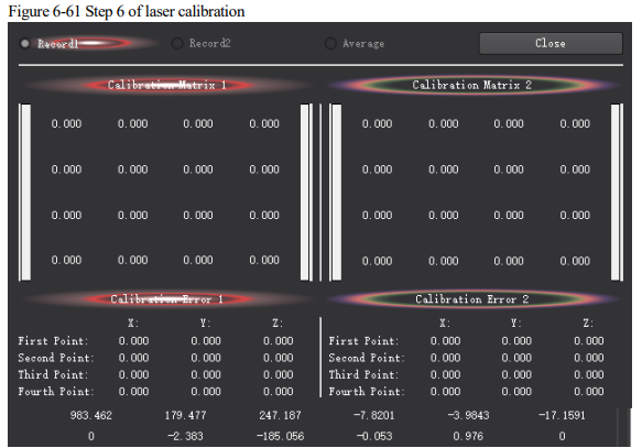
Step 6: Finally, click on "Next" after completing the Step 5. This will display the calibration matrix and error data.
Set the matrix to be used for calculations.
6.15.2 Laser Searching
Laser Searching refers to the process of using a laser to get the coordinates of a specific feature point and guiding the robot to reach that feature point.
You can perform laser searching tasks using the following two examples.
Example 1:

Example 2:

6.15.3 Laser Tracking
Laser Tracking refers to process of using a laser to get the position of a feature point on a section of a weld seam and directing a robot to weld that section.
Example:

Note:
In the example, as the robot moves to point P2, the laser system is already capturing welding seam
feature points. Once the robot reaches point P2, it begins to access the stored welding seam feature
points and continuously executes the welding operation until the laser system cannot detect feature
points or until it has completed the welding distance between P0 and P1.
6.15.4 Welding Adaptation
SetwelderThoughGap(3, 1, REAL0) //Plate thickness 3, and get the corresponding gap REAL0
By using the SetwelderThoughGap command, you can predict and measure various gap values along a weld seam. In the teach pendant's welding adaptation interface (refer to Figure 4-13), you can configure welding parameters based on these measured gap values. During the actual welding process, the system will automatically adapt the welding parameters according to the specific gap measurement, and get the appropriate welding scheme for each gap.
6.16 Calibration of User Coordinates/External Tool Coordinates
[Note]
In this section, the calibration operation of the user coordinates is illustrated. The calibration method for external tool coordinates is the same as the user coordinates. When modifying, the default name of the user coordinates is USERCOOR, while the default name of the external tool coordinates is EXTTCP.
Perform calibration to a user coordinate system by following the procedures below.
Step 1 Enter the program data interface, and click the user coordinates to be calibrated in the global scope, e.g. USERCOOR1, as shown in figure below.
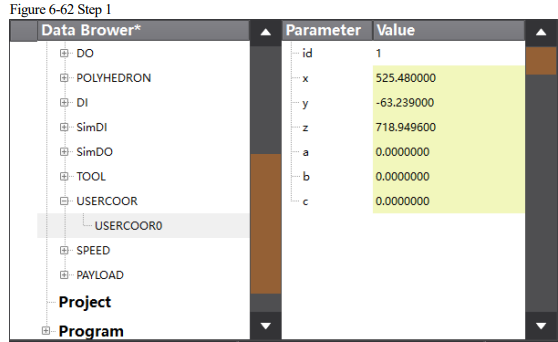
Step 2 Click "Modify" to enter the preview interface of user coordinates, as shown in figure below.
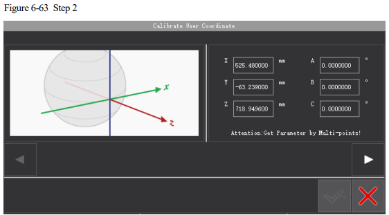
Step 3 Click "Settings" to enter the calibration method selection of user coordinate system.
There’s only the "3-point calibration method" available currently, as shown in figure below.
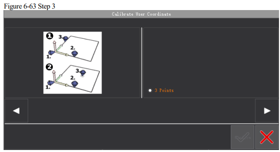
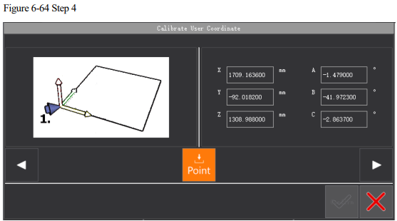
Step 4 Click "Next" to start teaching the coordinates at the origin, and move the robot to the origin of the user coordinates. By clicking "Teach", the interface will record the coordinates of the origin (the first point), as shown in figure below.

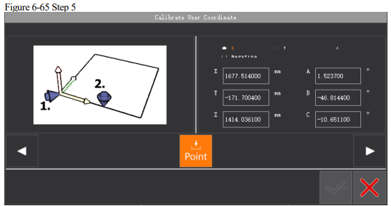
Step 5 Click "Next" to move the robot to any position on the X-axis of the user coordinate system. Click "Teach", the interface will then record the coordinates of the second point, as shown in figure below.
Step 6 Click "Next" to move the robot to any position on the XY plane of the user coordinates. Clicking "Teach", the interface will record the coordinates of the third point, as shown in figure below.
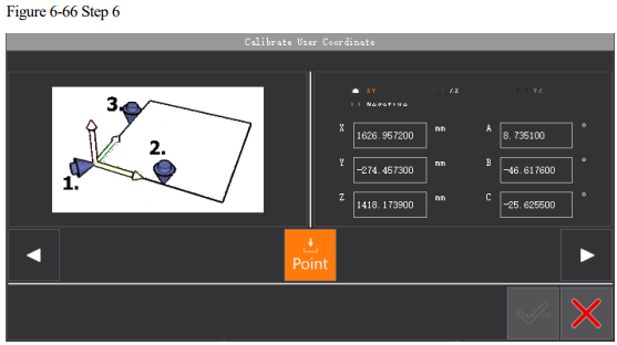
Step 7 Click "Next" and return to the preview interface of user coordinates, as shown in figure below.
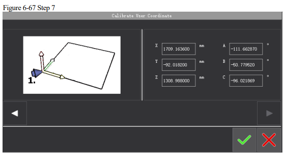
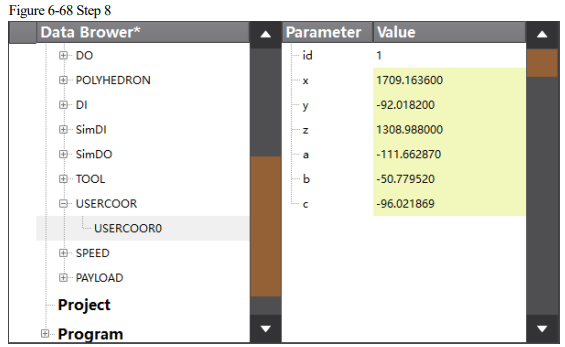
Step 8 Click "OK" after it is confirmed to be correct. The modification is finished, as shown in figure below.
6.17 External TCP
6.17.1 Function overview
Usually, the tool is mounted on the robot, and perform the specified tasks by tracking the motion of robot. In some specific applications such as gluing, it is required to install the glue gun (tool) at a position outside the robot, while the workpiece needs to be fixed on the robot for gluing. Such kind of tool mounted outside the robot and in a fixed position is called External TCP.
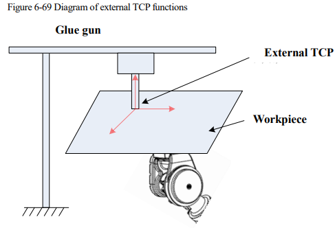
Calibrate the external TCP before using the external TCP functions. For details, please refer to "External tool coordinates".
The external tool coordinates may be selected in the jog reference coordinates. When the external tool coordinates is selected as the reference coordinates, the jog position and posture are relative to the external tool coordinates. The jog position under the external TCP is similar to the jog position under the user coordinates, and both move along the X, Y, and Z directions of the reference coordinates. The difference between the jog posture in the external tool and the jog posture in the user coordinates: for the jog posture in the user coordinates, the TCP point does not move, while the posture rotates around the TCP point. For the jog posture of the external tool, the TCP point rotates around the external tool coordinates.
In MovL and MovC commands, the reference coordinate system can be selected as external tool coordinates. The current reference coordinate system can also be set as external tool coordinates using the command SetExternalTCP. When the external TCP is used to teach linear and circular motions, teach 2 points in a linear mode, and 3 points in an arc mode.
[Note]
⚫ The posture point stored in teaching can be the description of the TCP point relative to the external TCP.
The motion of is relative to the external TCP coordinates.
⚫ For example, when external TCP functions are used, if the teaching origin and endpoint of the workpiece is attached to the external TCP origin, the contour of the workpiece is a straight line, irrespective of the changes of posture of the teaching origin and endpoint. When linear motion commands are used, the contour of the workpiece always moves along the external TCP origin. The motion speed is the speed of the workpiece relative to the external TCP coordinates.
6.17.2 Way of use
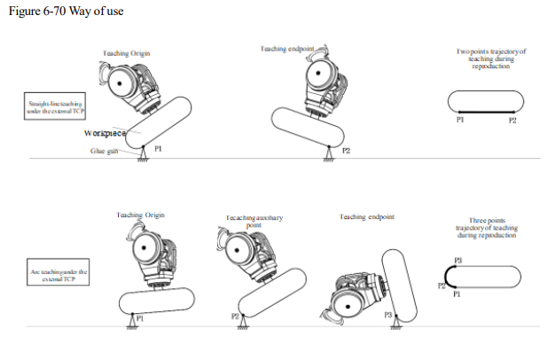
6.18 Single-point Alignment Coordinate Axis
6.18.1 Function overview
In some applications, the robot needs to rotate the posture so that a certain axis or full axis in the tool coordinates can accurately be perpendicular or parallel to the specified plane. In this case, the
Single-point Alignment Coordinate Axis would satisfy this requirement. Users may teach the target posture of the robot roughly, and then perform the precise gesture adjustment by using the Singlepoint Alignment Coordinate Axis so as to achieve the final target posture.
6.18.2 Way of use
Step 1 Enter the Jog Management group in the Home; click "Tool Alignment", and enter the operation interface of "Single-point Alignment Coordinate Axis", as shown in figure below.
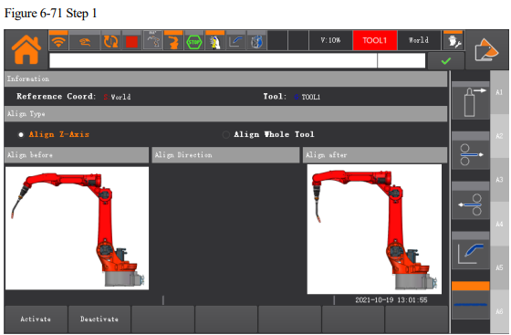
Step 2 Select the "Alignment Type".
⚫ Single-axis alignment: The alignment will be performed only to the Tz direction of tool coordinates and the nearest coordinate axis of the specified coordinates.
⚫ Full coordinate system alignment: Align each axis (Tx, Ty, Tz) of tool coordinates with the specified coordinate system.
[Note]
"Alignment" is an operation that will not change the current TCP position, but making the TCP be parallel to the axis of the specified coordinate system only by changing the posture.
Step 3 Click "Activate".
To cancel the alignment operation, click "Disable".
Step 4 Perform the alignment by clicking the "+/-" key corresponded to "GO" in the upper right corner.
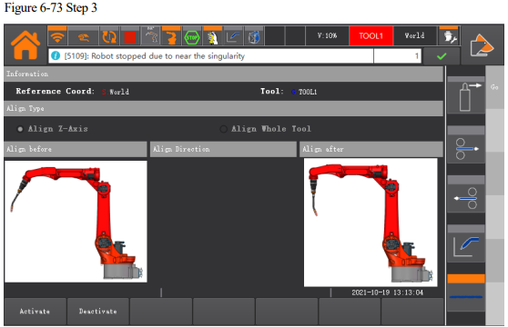
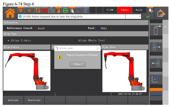
Step 5 A pop-up window means that the alignment is successful, as shown in the figure below.
6.19 Servo Management
6.19.1 Function overview
Users can directly clear and reset servo drive alarms, set some PN parameters, view servo version information, and perform batch backups and restores through the interface of the programming pendant.
[Caution]
⚫ Before performing "Servo management" operations, please confirm that the following conditions are met:
The axis drive numbers (Axis 1 to Axis 6) corresponding to the robot joints have been confirmed.
6.19.2 Way of use
Enter the General Settings group in the Home; click "Servo Management", and then enter the "Servo Management" operation interface, as shown in figure below.
6.19.3 Clear servo alarms
The "Clear Servo Alarms" operation interface is displayed by default when first entering the Servo Management page, as shown in figure below. You can also click the bottom function button to switch to the "Clear Servo Alarms" operation interface.
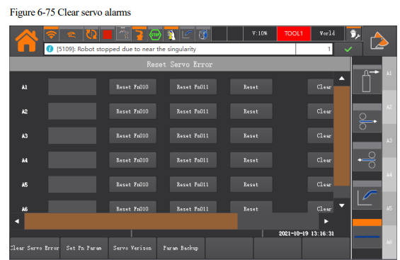
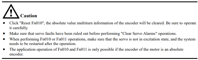
⚫ Click "Reset Fn010" and "Reset Fn011" to clear the servo alarms associated with the absolute encoder (A.45, A.46, A.47, A.48, A.51).
⚫ Click "Reset" to clear the current servo alarm of the right axis.
⚫ Click "Clear History Alarm" to clear the history alarm of the right axis.
6.19.4 Set PN Parameters
Click the "Set PN Parameters" function button at the bottom to enter the "Set PN Parameters" operation interface, as shown in figure below, which initially displays the PN parameters of Axis 1.
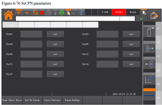
⚫ Click the "Set PN Parameters" function button at the bottom to get the PN parameters of current axis on the interface.
⚫ Click the corresponding axis number tab to get the PN parameters of the corresponding axis.
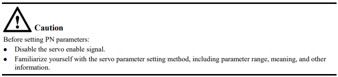
⚫ Clicking the "Set" button for the corresponding PN parameter pops up an input box. After entering a value, click the "OK" button to send the input value to the servo. After the setting is done, the current PN value is displayed in the corresponding PN parameter textbox.
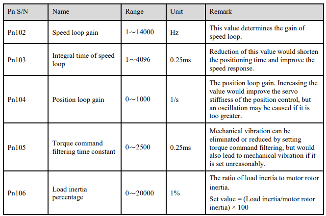
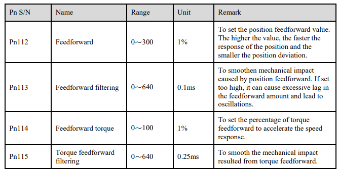
6.19.5 View Servo Software Version
Clicking the "Version Information" button at the bottom will take you to the "Servo Software Version" screen, as shown in figure below.
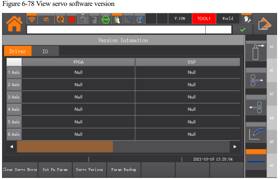
⚫ After the teach pendant is started normally, clicking the "Version Information" button at the bottom will obtain the servo software version and display it on the screen.

6.19.6 Servo Parameter Backup & Restore
Clicking the "Backup & Restore" button at the bottom will take you to the operation screen for "Servo Parameter Backup & Restore," as shown in figure below
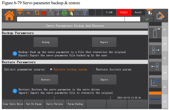
⚫ Clicking "Backup" will prompt for a password. Use the administrator password to confirm the operation. After the password is verified, the controller will locally backup the current portion of the Pn parameters. Note that the backup file will overwrite the original backup file.
⚫ The restoration of servo parameters can be divided into two types: restoring user-backed up parameters and restoring factory-backed up parameters. Select the type of backup to restore using the radio button.
⚫ Restoring user-backed up parameters: i.e., restoring servo parameters backed up or imported by the user.
⚫ Restoring factory-backed up parameters: When the machine is delivered, a servo factory parameter backup file is provided for each model. Restoring this backup file will restore the parameters to the servo.
⚫ After selecting the backup type using the radio button, click "Restore" and enter the password. Use the administrator password to confirm the operation. After the password is verified, the controller will execute the restore operation.
⚫ Insert a USB flash drive and click "Export" to download the user backup parameter file to the root directory of the USB drive.
⚫ Insert a USB flash drive and click "Import". Enter the password, use the administrator password to confirm the operation, and after the password is verified, select the imported servo backup parameter file.
[Caution]
⚫ The servo must be disabled before performing backup and restore operations.
⚫ Performing "Backup" and "Import" operations will overwrite the original backup file. To preserve the original backup file, use the "Export" function.
6.20Use of 2D vision
6.20.1 Function overview
Robot vision refers to the system that provide the robot with visual perception function. It is one of the key parts of the robotic system. Robot vision can obtain a 2D image through a vision sensor, make analysis and interpretation using a vision processor, and then convert it into a symbol, so that the robot to recognize an object and know its location exactly.
6.20.2 Way of use
The 2D vision setup screen is shown in figure below.
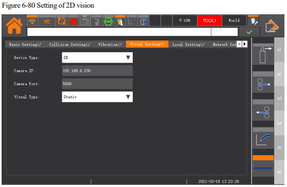
Select System Home → General Settings → Visual Settings to enter this interface.
Select "2D" for the "Camera Device Type" option. Fill in the "Camera IP" and "Camera Port
Number" according to the actual parameters, which are set to 192.168.6.230:5000 by default.
Currently, only static visual types are supported.
6.21 Use of 3D vision
6.21.1 Function overview
Robot vision refers to the system that provide the robot with visual perception function. It is one of the key parts of the robotic system. Robot vision can obtain a 3D image through a vision sensor, make analysis and interpretation using a vision processor, and then convert it into a symbol. It is used to set the robot's variables, position points, and IOs. Also, it needs to get the robot's variables, position points, IOs, current position and other commands, to enable the robot to recognize objects and be controlled by visual logic.
6.21.2 Usage I
The robot is the client, while the vision device is the server.
The 3D vision setup screen is shown in figure below.
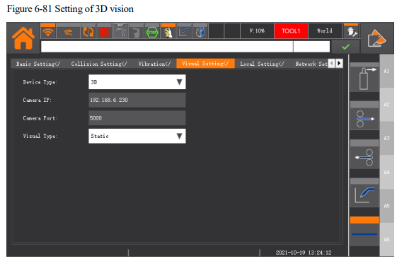
Select System Home → General Settings → Visual Settings to enter this interface.
Select 3D for the camera device type. Fill in the camera IP and port number as per the actual parameters. It is defaulted as 192.168.6.230:6000
The vision type does not work in 3D mode.
Send a character string to the vision settings by using the command SendMessage. The content of the character string can be defined by the user. For example, sending the string "ScanReque" to the camera can be achieved by executing SendMessage("ScanReque",1).
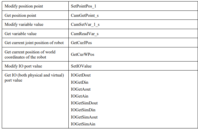
Vision obtains 3D images of the environment using the sensor, makes analysis and parsing, and then converts them into vision commands to set or get robot variables, position points, IOs, etc.
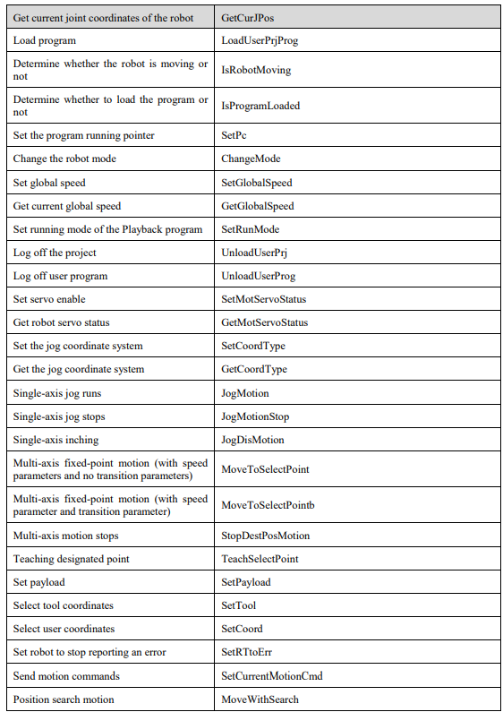
The vision commands on the robot are listed in table below.
6.21.3 Usage II
Using robot as the server, and the vision device serves as the client. The robot server is configured as follows:
⚫ IP: 192.168.6.63 (controller’s IP address)
⚫ Port: 5000
Step 1 Establish the connections.
1. Controller internally start the python script to create the server-side.
2. Configure the client device to make it connect to the robot. (Ping the controller IP 192.168.6.63)
3. Configure the client device to use the above connection parameters.
4. Establish a connection with the server. (The client should send a read and write request to the server every 10 seconds at the moment to keep the connection as a heartbeat)
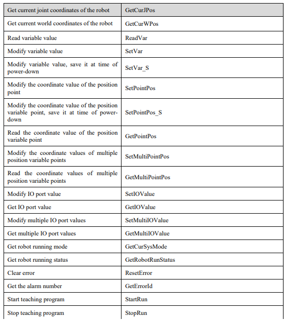
Step 2 The vision client then sends commands to the server.
The vision commands sent to the robot are listed in table below.
6.22 ModbusTCP
6.22.1 Function overview
ModBusTcp protocol interface is a communication mode in which an external logic controller (PLC, etc.) communicates with the robot via the standard industrial bus protocol (ModBusTCP), and reads and writes the virtual IO port of the robot. The robot can interact with external devices through ModBusTCP without additional expansion of IO ports.
ESTUN robot controller, as a server, provides the following functions to external control device through ModbusTCP protocol:
⚫ Access and control virtual I/O;
⚫ Read the current robot running status;
⚫ Start/stop the program using the control word, enable the robot, load/log off the program, set the global speed.
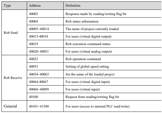
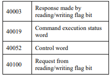
The ER series robot encapsulates a layer of data structure in the ModBusTCP holding register, as listed in table below.
6.22.2 Way of use
The ModBusTCP interface of ER series robots is configured as follows:
⚫ IP: 192.168.6.68 (real-time system IP address)
⚫ Port: 502
⚫ Cycle of collection >50ms
⚫ Response timeout>100ms
⚫ Heartbeat time <10s
Step 1 Establish the connection.
1. Configure the client device to make it connect to the robot. (Ping the real-time system at IP 192.168.6.68)
2. Configure the client device to make it use the above connection parameters.
3. Establish a connection with the server. (The client should send a read and write request to the server every 10 seconds at the moment to keep the connection as a heartbeat).
Step 2 Read and write SimIO.
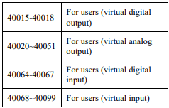
According to the table below, the virtual output is SimOutput. The client should read the value of the corresponding register, and map it to the input of the external device. The virtual input is SimInput. The client should write the value to the corresponding register, and then map it to the output of the external device.
Step 3 Read the robot status.
The 40004 register of the server is of the robot status word. 40002 is the current global speed of the robot.
The table below lists the meaning of each bit of the robot status word:
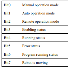
The client can read the corresponding Bit through the mask to get the robot status.
Step 4 Send the control commands.
Send commands such as starting/stopping program, loading/logging out program, and setting global speed to the robot as per the procedures below.
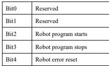
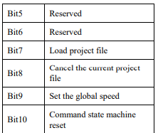
1. Reset the command execution interface by writing the command control word 40052 as 0, and 40100 as 0.
2. Write 40100 as hexadecimal 0x11.
3. When the value of 40003 is 0x11, set the corresponding Bit of the control word according to the table below.
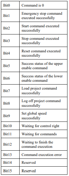
4. When the corresponding bit of the command execution status word 40019 is 1, it indicates that the command is executed successfully.
5. When 40100 is 0, it means that 40019 is reset.
6.23 Lockup and Unlock
The robot lockup refers to the time range set for the robot's use authority by using this application program. The robot can operate normally in such time range. If it goes beyond such time range, the robot will then stop working by locking the motion.
The robot can be in four lockup states: The locked state of robot, the unlocked state in stage 1, unlocked in stage 2, unlocked in stage 3, and unlocked indefinitely.
No lockup setting is made for the robot at time of delivery, but be defaulted to unlock indefinitely.
Once it has been locked up, the motion and other related operations cannot be performed.
The number of days of lockup are to be set and cleared by the manufacturer by entering a dynamic password to log in. The unlocking operation can be done by the user after getting the unlocking key from the manufacturer.
6.23.1 Turn on lockup management application
Use "User" or above to log in to the teach pendant, and switch to the "Advanced Settings" subgroup interface in the System Home Page, and click the Lockup Management button to open the Robot Staging Lockup Management application interface, as shown in the figure below.
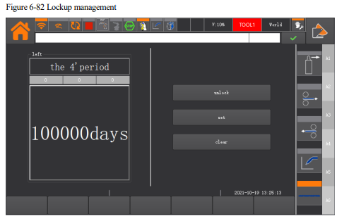
⚫ Remaining: Display the current period type and the remaining days of the current period. If the "special period” is displayed for the permanent unlocking, the remaining days are "indefinite period";
⚫ Unlock: Open the period unlocking interface. This operation can be finished by users.
⚫ Setting: Open the interface for setting the period of days. The operations in this interface can only be performed by the manufacturer’s personnel after entering the dynamic password.
⚫ Clear: Open the permanent unlocking robot setting interface. The operations in this interface can only be performed by the manufacturer’s personnel after entering the dynamic password.
6.23.2 Set lockup period
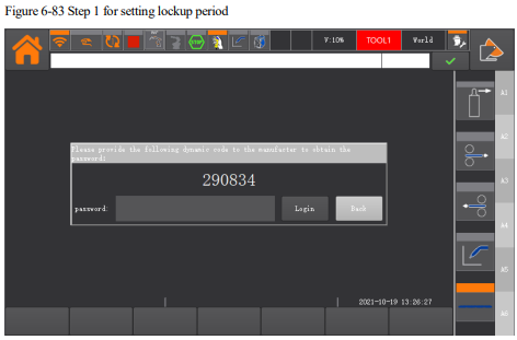
Step 1 Open the lockup management application interface; click the "Set" key. The teach pendant is displayed as shown in figure below. According to the prompt dynamic code, the manufacturer's personnel can then obtain the login key and log in.
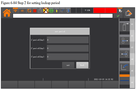
Step 2 After logging in, as shown in figure below, enter the restricted number of days for stages 1, 2, and 3, and click the "Set" key to invalidate the set days.
[Note]
⚫ After the robot software is mounted at time off delivery, and if the lockup is not configured, the lock will be not restricted by default, and all the functions can be used permanently.
⚫ All the days for the three stages need to be filled in, and be invalid after setting.
⚫ After setting, the stage 1 lockup will be valid. The starting time is the current time of unlocking.
6.23.3 Unlocking period
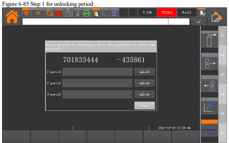
Step 1 Enter the staged lock management application interface, click the "Unlock" button, and the teach pendant will display as shown in figure below. Then, provide the machine code and the number of stages to be unlocked to the manufacturer to get the unlocking key. The machine code consists of two parts, and the format is: fixed codedynamic code.
Step 2 After unlocking the appropriate period, the period will then become valid. You can refresh to view the current remaining days in the corresponding interface.
[Note]
⚫ The current number of days after unlocking will become valid immediately. The start time will be the current unlocking time.
⚫ If unlocked in an early time, only the number of days in the current period will be valid, and the days in the previous period will be invalid by default.
6.23.4 Clear lockup period
Step 1 Enter the staged lock management application interface, click the "Clear" key, and the teach pendant will display as shown in figure below. According to the prompt dynamic code, the manufacturer's personnel can then obtain the login key and log in.
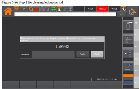
Step 2 Log in the lockup clearing setting interface, as shown in figure below. According to the prompt machine code, the manufacturer's personnel is provided with the clearing key
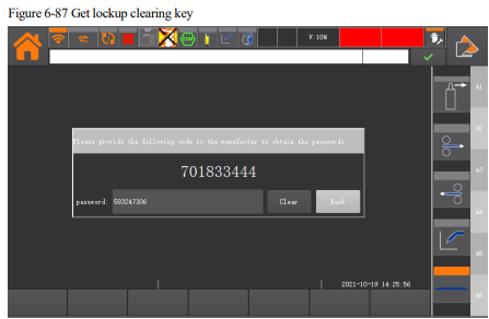
Step 3 After the lockup function is cleared, the robot enters an unlocked state indefinitely. You can refresh and view the current period in the interface of remaining days with no "Special Period" displayed, and the remaining days are "Indefinite".
6.24 SoftFloat
6.24.1 Function overview
SoftFloat functions are used for extracting workpieces from the die-casting machine. The SoftFloat functions of the robot works to turn the robot into a flexible body. The robot can move in response to changes in the external force under the action of external forces to prevent damage to the robot and workpieces resulted from the rigid contact. This allows the realization of linear SoftFloat functions in the specified direction. The robot can perform the linear motion following the diecasting machine ejector rod.
⚫ When the workpiece is gripped by the robot and the machine is performing feeding/blanking operations, there is a difference between the gripping position and the final position of the rough workpiece. Linear SoftFloat function works to change the robot from a rigid state to a flexible state without using external sensors or adding a mechanical construction. The end of the robot can move in a straight line in the specified direction under the actions of the external force, and fit the workpiece well to avoid collision and friction. The function is used in die-casting and other workpiece feeding/blanking operations.
⚫ When SoftFloat is started, the motion speed of robot is determined by the external force. The greater the external force, the faster the robot will move.
⚫ SoftFloat function can be started by following modes:
Auto running (single-step, continuous)
Manual running (single-step, continuous)
Caution
⚫ When using SoftFloat functions, please specify the correct SoftFloat direction to ensure that it is consistent with the moving direction of the workpiece.
⚫ After SoftFloat is turned on, the following situations occur, and SoftFloat functions are turned off.
→The controller reports an error
→When the stop button or E-stop button is pressed
→SoftFloat is turned on for more than the waiting time of system settings
⚫ The starting and closing commands of SoftFloat need to be used together, of which the starting command shall be set before the closing command. If you want to execute multiple groups of SoftFloat functions in a teaching program, multiple sets of start and ending commands shall be set. The control system will report an error when the following commands are set.
→Only executing the SoftFloat starting command
→Only executing the SoftFloat closing command
→Executing the SoftFloat closing command before the starting command
→Executing the SoftFloat starting command continuously
⚫ The control system will report an error if the action commands are inserted into the SoftFloat starting and closing commands.
⚫ Never use SoftFloat functions near the singular point.
⚫ Stop the SoftFloat after the external force is removed, in such a way that the robot will stop without producing vibration.
⚫ If the last motion command of the SoftFloat starting command contains transition information, no transition processing will be performed.
⚫ When SoftFloat is turned on, the collision detection and maximum torque detection functions are turned off, which will be restored when SoftFloat closes or an error is alarmed after SoftFloat functions is turned on.
The SoftFloat direction can be set by following the procedures below:
Before extracting workpieces using SoftFloat, confirm whether the SoftFloat direction is set correctly. When tool coordinates are selected as the reference coordinate system, the linear motion direction will be the direction of tool coordinates direction selected at the start point of SoftFloat.
The direction of SoftFloat tool coordinates is the same as the direction when the robot is in jog operation. When TOOL is selected as the reference coordinate system, the coordinate system number shall be nullTool. When the Y direction is selected for SoftFloat, the direction of the linear SoftFloat is shown as follows:
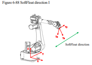
The flexibility effect will the best when the direction of SoftFloat is set in parallel to the tangential direction of the horizontal rotation of the robot's force point around the Z-axis of the world coordinates; when the angle θ is greater than 60 degrees, the linear SoftFloat will report an error.
The angle θ is the angle between two straight lines in space. It is illustrated as follows:
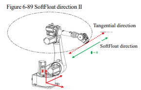
The flexibility will be better if the angle between the tangential direction is parallel to the SoftFloat direction.
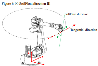
The flexibility will be poor if the angle between the tangential direction and the SoftFloat direction is larger.
6.24.2 Application example
The extraction of workpieces from the die-casting machine will be taken as an example. The field application of SoftFloat can be in following process:
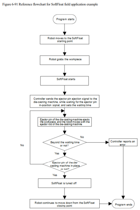
When the program runs to the starting point of SoftFloat, the workpiece will be gripped first. After the SoftFloat is turned on, the controller sends DO signals to the die-casting machine, while waiting for the DI signal input of the die-casting machine ejector in-position signal and setting the waiting time. When the die-casting machine receives the DO signal, the die-casting machine ejects the ejector rod, and the robot can move by following the ejector pin; When it goes beyond the set waiting time, the controller alarms. The SoftFloat ends when the controller receives the ejector inposition signal. The robot continues to move down from the position where the SoftFloat ends.
Example of teaching:
MovJ(P0,V100,"RELATIVE",C0)/*Robot moves to the SoftFloat starting point P0*/
SetDO(DOO,0) /*Control the gripper to grasp the workpieces*/
Wait(500) /*Wait for 0.5s*/
SoftFloatStart(CART,TOOL,nullTool,Y,LOW) /*After the linear SoftFloat is turned on, the robot can move in a straight line along the Y direction of tool coordinates without tool parameters, and the
SoftFloat flexibility level is LOW*/
SetDO(DOO,1)/*Send out the die-casting machine ejector pin moving forward signal*/
WaitDI(DIO,0,8000,0,INT0) /*Controller waits for the in-position signal of the ejector pin of the die-casting machine and sets a waiting time of 8s, then returns to the in-position signal state INT0*/
IF INT0.value >0 THEN/*Judge if it is in position*/
SetRtToErr("WaitError",10000)/*Controller reports an error if it is beyond the set waiting time for
8s*/
ENDIF;
Wait(500) /*Wait for 0.5s till the robot stop moving; the waiting time depends on the actual conditions*/
SoftFloatStop()/*SoftFloat function is turned off */
MovJ(P1,V100,"RELATIVE",C0)/Robot moves from the SoftFloat endpoint to point P1
6.25 9-point Calibration
6.25.1 Function overview
9-point calibration is designed for the field applications of ESTUN robots equipped with camera vision device. With this function, the camera can send directly the pixels of the object being shot.
After the robot controller receives the camera pixels, they can be converted into the position points under world coordinates internally. The robot is allowed to grasp accurately the target object based on the position points converted.
6.25.2 Way of use
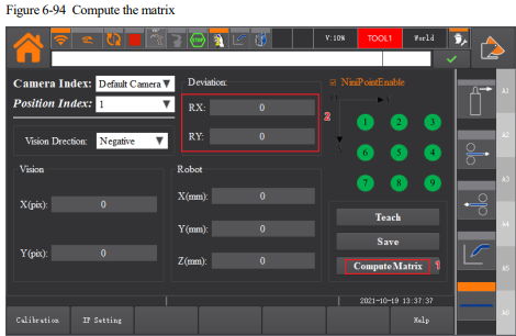
Step 1: On the System Home, select "User Applications > 9-point Calibration" to enter the corresponding operation interface, as shown in figure below.
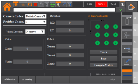
Step 2 Set the vision coordinates and robot coordinates.
Put the calibration paper under the camera, and make sure that the 9 calibration points are within the shooting range of the camera. After shooting, 9-pixel position points will be produced, which shall be recorded. Then operate the robot manually, move the TCP points of the robot to positions 1~9 on the calibration paper in turn. Each time when the robot moves to a calibration point, enter the corresponding pixel coordinates into the visual box, and then click
Teach to display the robot coordinate points, and finally click “Save” button. This shall be done from 1 to 9 on the calibration paper.
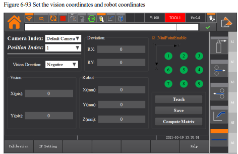
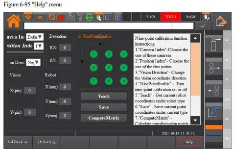
1. Select the corresponding camera; each camera shall have the appropriate calibration parameters.
2. The initial interface is not operable; check the upper right corner to enable 9-point calibration function.
3. Operate the teach pendant manually to move the robot to calibration point 1; select point 1 and input manually the pixel position corresponded to the calibration point 1; keep the robot TCP point coincident with point 1 on the calibration paper, and then click to teach the current robot coordinate point. Click “Save” key.
4. Repeat the above operation, select calibration points 2~9 in turn, and input the pixel position points corresponded to the calibration points; click “Save” after each time of input.
[Note]
⚫ Selection of calibration direction: Select the positive direction when the Z direction of the camera working coordinates is the same as the Z direction of the world coordinates, the positive direction is selected here; and select negative when the Z direction of the camera working coordinates is opposite to the Z direction of the world coordinates.
After each point has been taught, click the “Save” button.
⚫ Compute the matrix.
Click the “Compute” button after setting the visual pixel position point and robot coordinate point. The computation error is displayed at RX and RY, and the normal error is within ±0.1. After computation, keep the 9- point calibration enable in the enabled state. Then, send the shot target object point to the robot end using the camera to observe if the robot can move to the target object correctly
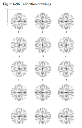
⚫ Calibration drawings
The serial number of the calibration point of the vision and robot must be the same as the figure below.
6.26 Positioner
6.26.1 Function overview
With the positioner function, the workpiece can be moved to a suitable position for welding upon the rotation and flip of the worktable. It also makes collaborative motion with the robot so as to improve the production efficiency and welding quality.
Up to 6 positioners can be configured. 1-axis rotary positioners and 2-axis rotary positioners are supported.
Note: In the screenshots of this chapter, the axis name "Ex" is equivalent to "PEx".
6.26.2 Calibration of positioner coordinate system
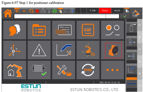
Step 1 Click "Positioner" in the "User Application" plug-ins on the Home interface, as shown in figure below.
Step 2: Select the "Positioner ID" to be set, for example, selecting positioner ID = "1".
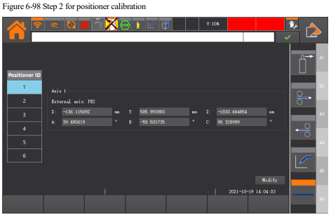
Step 3 Click "Modify" to set the coordinate system of positioner ID=1.
The positioner coordinate system can be determined by inputting or by calibration.
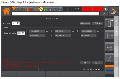
Step 4 Set the "Number of Axis" as needed.
⚫ It is defaulted as "1", indicating 1 additional axis. User only needs to calibrate one additional axis.
⚫ It indicates 2 additional axes if set it to “2”. User needs to calibrate the 2 additional axes.
When the number of axes is set to "2", select the additional axis to be calibrated by clicking "Switch Axis".
Caution
When 2 additional axes are set, make sure that the additional axis corresponded to the second axis of the positioner is at the zero position when calibrating the "1-axis coordinate system"; vice versa.
The additional axis corresponding to axis 1 of the positioner should be selected from the base axis of the positioner.
Step 5 Select "Additional Axis", and then click "Calibrate".
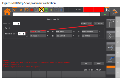
Caution
During calibration, make sure that the axis of the positioner teaches by rotating in the positive direction, and keep
the other axes of the positioner at the zero position.
Step 6 Select the model of the positioner, e.g. "Model 1".
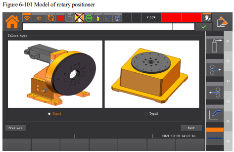
[Note]
For the model 3 corresponding to the "3-axis positioner", it can be configured as two two-axis positioner.
Step 7 Click "Next" to teach the positioner at three points.
[How to calibrate]
1. Install a point device or find a characteristic point prior to calibration as a marked position.
2. Move the robot TCP to such position, and then click "Teach".
3. Click "Next" and continue to rotate the positioner axis to an angle (recommended greater than 30°), move the robot TCP to the marked position, and then click "Teach".
4. Click "Next", and after rotating the positioner axis to the angle (recommended greater than 30°) for the second time, move the robot TCP to the marked position, and then click "Teach".
5. Click "Next", and the calibration "result" will appear.
Step 8 Click "OK" after they are confirmed to be correct.
[Note]
When calibrating the "2-axis coordinate system", make sure that the additional axis corresponded to the 1- axis of the positioner is at the zero position. Then, click "Switch Axis", and calibrate the 2-axis coordinate system with the same method.
Step 9 After returning to the positioner coordinate system interface, click "OK", and the positioner ID=1 coordinate system is successfully calibrated.
6.26.3 Use of positioner coordinate system
Before the positioner coordinate system is used, it is necessary to create a POSITIONER variable,
and specify the parameter index as the correct positioner ID. This can be done in two ways:
⚫ Use the command "SetPositioner" directly, which indicates to switch the system coordinate system to the positioner coordinate system.
⚫ When following motion commands are used, set the "Coordinate System Parameter" to the specified Positioner variable.
MovL, MovC, MovLRel, MovLSearch, MovH, MovLW, MovCW.
6.26.4 Application example
The left and right sides of the robot are provided with a positioner each. The robot first performs synchronous motion with the U-shaped positioner on the left (variable POSITIONER1 has been set), and then with the L-shaped positioner on the right (variable POSITIONER0 has been set). The structure of command is shown in figure below.
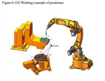
The executing commands are detailed as follows.
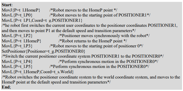
6.27 Execution in Reverse
6.27.1 Function overview
This function is introduced if sometimes it needs to return according to the original track to avoid collisions, etc. when the program executes the complex motion commands. In the above situation, execution in reverse is required, so as to return to the original track.
In the reverse mode, the motion commands that are allowed for execution in reverse will perform such operation, and alarms will be given for the motions or other commands that are not allowed.
Other commands that do not affect the return of the original track will be skipped and not executed.
6.27.2 Way of use
In manual mode, press the  key to enter the Execution in Reverse mode, and press the
 key again to return to the positive sequence mode.
Caution
Followings shall be noted when using this function.
⚫ After the program is logged off or loaded, it is automatically restored to execution in positive sequence.
⚫ The reverse execution is limited to single-step execution performed manually.
⚫ When using this function, skip directly for any skippable commands, which will not be executed.
⚫ When using this function, the system will give an alarm in case of an unexecutable command.
⚫ When performing execution in reverse, the commands such as SetPC will lead to changes in the running path.
This is a manual intervention, while the risk is to be borne by the operator.
⚫ The reverse function cannot be performed by crossing programs. It does not support calling back to the main program from the CALL program.
The executable and skip-able commands during reverse execution are shown in Table 7-10. Any commands not listed are unexecutable.
[Note]
The END line or the commented command line as well as the comment line or Label command line are all skippable by default.
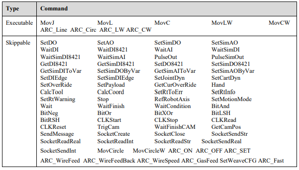
6.28 Servo Parameter Self-tuning
6.28.1 Function overview
The servo parameter self-tuning function is designed to improve jittering during various robot applications during low-speed running. It can also reduce the large position error caused by jittering. By setting corresponding parameters, the best effect can be achieved in various speed ranges.
⚫ The servo parameter self-tuning function is mainly used to improve the low-speed shaking phenomenon of the robot within a certain speed range. To enable this function, use the command "AutoGainEnable()" and set the following parameters: gain ratio threshold and speed range threshold.
⚫ The gain ratio threshold (LsScale) is set for each joint axis, with a range of [100, 1000], in %.
⚫ The speed range threshold (LsThresh) is set for each motor axis, with a range of [10, 1000], in r/min.
⚫ The servo parameter self-tuning process depends on servo parameter Pn104. If Pn104 is modified, there may be slight differences in the effect when using the same parameter (gain ratio threshold) before and after the modification.
⚫ To disable the servo parameter self-tuning function, use the command "AutoGainDisable()".
Caution
⚫ To enable the servo parameter self-tuning function, the following conditions must be met:
→The enable item must be configured in the EAxisParam.ini configuration file.
→The corresponding servo parameter file AutoGainServoParam.json must be configured in the configuration folder.
⚫ The servo parameter self-tuning function is not enabled by default.After the command is executed, the host program logs off/executes the OFF command to turn off the function
6.28.2 Application example
When the program executes the "Servo parameter self-tuning function" start command, the function is enabled. Once enabled, the controller will automatically adjust the corresponding servo parameters. If the set command parameter value exceeds the maximum limit, the controller will issue an alarm.
Example of teaching program:
./*Program execution section, servo parameter self-tuning function disabled by default */
.
.
AutoGainEnable(LsScaleP=t_g.LsScale0,LsThreshP=t_g.LsThresh0)/*Enable the servo parameter self-tuning function*/
.
.MovL(P1) //The controller will automatically adjust the servo parameters when executing this motion command
AutoGainDisable()/*Disable the servo parameter self-tuning function */
6.29 Cross-wrist Singularity
6.29.1 Function overview
The Cross-wrist Singularity Function enables the robot to traverse through the wrist singularity point (when J5=0, wrist singularity occurs) along the taught path, thereby improving the robot's motion space. However, the cross-wrist singularity function cannot guarantee the orientation of the robot during path motion.
Cross-wrist singularity function can be turned ON or OFF via command.
⚫ The SetSingularPass ("string") is used to set the switch of the cross-wrist singularity function.
⚫ Cross-wrist singularity function.The string can be "OPEN" or "CLOSE". When "OPEN" is selected, the crosswrist singularity function is turned on, and when "CLOSE" is selected, the function is turned OFF.
Caution
⚫ When the wrist singularity function is enabled, the robot's posture during the teaching path cannot be guaranteed. Therefore, execute the motion slowly to prevent robot collision;
⚫ Even if the user selects the cross-wrist singularity mode, the robot will move according to the non crosssingularity mode if the current segment does not cross the wrist singularity;
⚫ The cross-singularity function is only applicable to universal six-joint robots with wrist singularity and does not support other robot types or other singular positions;
⚫ The cross-wrist singularity function supports the transition between motion commands, but the SetSingularPass command interrupts the transition;
⚫ JOG mode does not support cross-singularity;
⚫ Swing motion, tracking motion, and external TCP functions do not support cross-singularity;
⚫ The function supports the start point in the singular position, but not the end point;
⚫ Upon logout or loading of a project, the cross-singularity function will reset to its default value.
6.29.2 Application example
When the command for cross-singularity function is executed, the function is turned ON. If the cross-singularity OFF command is not executed, the function remains ON.
Example of teaching program:
Start:
SetSingularPass("OPEN")/*Turn ON the cross-wrist singularity function */
MovJ(P0);
MovL(P1); /*If the motion from P0 to P1 does not cross the singularity or only crosses the wrist singularity, the robot moves to P1*/
MovC(P2,P3); /*If the motion from P1 to P3 does not cross the singularity or only crosses the wrist singularity, the robot moves to P3 */
SetSingularPass("CLOSE")/*Turn OFF the cross-wrist singularity function */
End;
6.30 Homing
6.30.1 Function overview
The Homing calibration is an operation that compares the robot's position with the absolute encoder position. The Homing operation is usually performed before leaving the factory. However, in the following situations, the home position may be lost and the Homing calibration must be performed again.
⚫ Replacement of motors or absolute encoders resulting in loss of home position information;
⚫ Loss of home position information due to encoder battery failure or other reasons;
⚫ Other situations.
As shown in figure below, the following diagram illustrates the state of lost home position information (unRef: Home position information is lost):
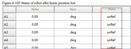
Caution
⚫ The operations in this Chapter only apply to the second situation mentioned above where the device is not replaced and the home position needs to be recovered due to encoder battery failure or other reasons. For other situations where components are replaced, home position must be recovered using instruments or other calibration methods.
⚫ The system provides two homing methods: Global Homing and Single-Axis Homing.
6.30.2 Global Homing
Global homing allows all axes in the robot axis group to perform homing at the same time, which generally causes some loss of accuracy. It is only recommended for applications where accuracy is not critical, as shown in figure below.
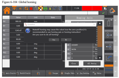
6.30.3 Single-axis homing
Single-axis Homing is a method of performing homing by using a one-key homing or RefRobotAxis command on the corresponding axis. This method can ensure the original accuracy of the robot and is recommended for use in applications.
Step 1: Jog the robot axis to the vicinity of the zero mark on the body of the corresponding axis, as shown in figure below.
After the robot is calibrated, the position of the waist hole for attaching the zero-mark sticker (labeled as "2") will be adjusted to align with the line labeled as "1". The single-turn absolute value data information for each axis will also be archived. This value can be viewed in the "Set Single Turn Value" in the "Single Turn Value" interface in the JOG interface.
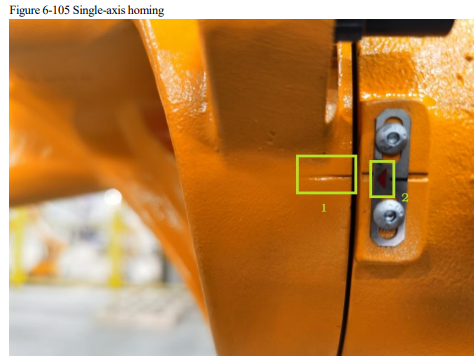
Caution
⚫ The arrow at point 2 should be jogged as accurately as possible to align with the line at point 1. If the line at point 1 is too wide, pay attention to whether the arrow passing through the area of the line at point 1 will cause the single-turn value of the corresponding axis to cross one turn (for example, from reaching the maximum value of 20,000 pulses to crossing 20,000 pulse value again). If the line at point 1 causes the single-turn value to cross one turn, there may still be accuracy loss issues even if the axis is homed in single-axis mode.
Step 2: Edit RefRobotAxis command, specify the axis number which needs to home, and fill the factory-set single-turn value data into the command parameters. In the interface of "Point Management->Position Management", select the item of "Single-turn Value" to view the value information recorded during factory calibration, as shown in the figure below.
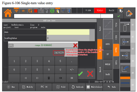
It can be read from the single-turn value Information section of the location management interface
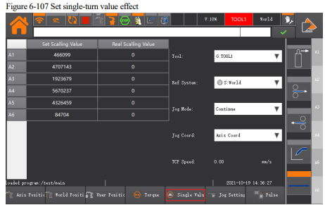
Caution
⚫ When there is coupling between joints, it's important to consider the homing sequence, starting with the source axis of the coupling. For example, if there is coupling between joints 4, 5, and 6 (4 couples with 5 and 6, and 5 couples with 6), the homing sequence should be 4 -> 5 -> 6.
Step 3: Run the RefRobotAxis command (the robot axis will move to the single-turn value position and perform homing operation).
RefRobotAxis (1,2419239)
/*The robot axis 1 will perform zero calibration at the position of 2419239 for a single-turn value when executing this command. */
6.31 Zero Loss Protection without Limit Block
6.31.1 Function overview
⚫ This function provides protection for the internal cables of the robot when the robot is not equipped with mechanical limit blocks and the zero point is lost during the homing process.
⚫ When the robot (no limit block) axis loses its zero point, the programming pendant position interface displays the robot's position before the loss of zero, as shown in figure below. Use this position as a reference for jogging and perform the Homing operation accordingly
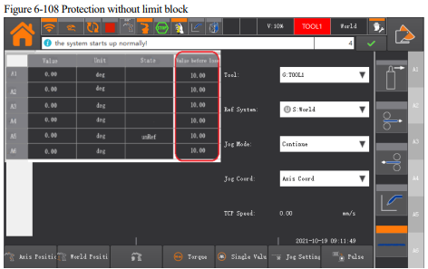
[Note]
⚫ The Zero Loss Protection without Limit Block function for the Axis 4 in the universal 6-axis robot is enabled by default;
⚫ After the Zero Loss Protection without Limit Block is enabled, and if an axis without limit block loses its zero point, the Programming Pendant Position Interface will display the position of each axis before zero loss. If other axes suffer zero loss, rather than those provided with no limit block, the teach pendant interface will not display the position of each axis before the loss of zero.
Caution
⚫ The position displayed on the teach pendant before zero loss may not be accurate in the following situations:
1) The controller software has been replaced;
2) The robot loses its zero point during high-speed motion;
3) The robot loses its zero point after an abnormal power-off restart during motion;
4) Move the joints manually after the robot loses its zero point.
6.32 Homing by One-Click
6.32.1 Function overview
⚫ In some applications, it is necessary to frequently return the robot to a specific position to check if the robot position has shifted. This function allows users to select and run the robot to a specified position through the interface.
⚫ The function interface displays the current position and target position, and supports two optional original positions that can be taught or modified.
⚫ After selecting the target position, click "Go" and keep it pressed down. The robot starts to move to the target position in a MovJ manner. Release "Go" during the movement to stop the robot, and click "Go" again to continue the movement until it reaches the target position.
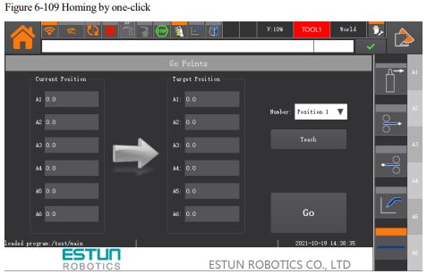
[Note]
⚫ Only the robot body axes are displayed during the homing operation.
⚫ The homing operation requires servo enablement and can only be performed in teaching mode.
⚫ Press the Rob key on the programming pendant to take you quickly to the Homing interface.