10. Tuning

10.1 Overview
10.1.1 Basic Conception
Tuning is the process of satisfying the servo performance by adjusting the parameters involved in the
control law.

Tuning Flow
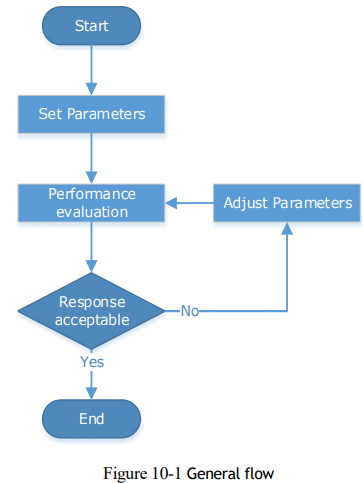
The process of tuning is usually an iterative process, and Figure 10-1 shows the general flow. 

Parameter Classification
There are two types of parameters in the tuning.
 Function Parameters: refers to some application function selections or switches that may improve Servo performance.
 Adjustment Parameters: increasing or decreasing these parameters may improve Servo performance.

Servo Performance
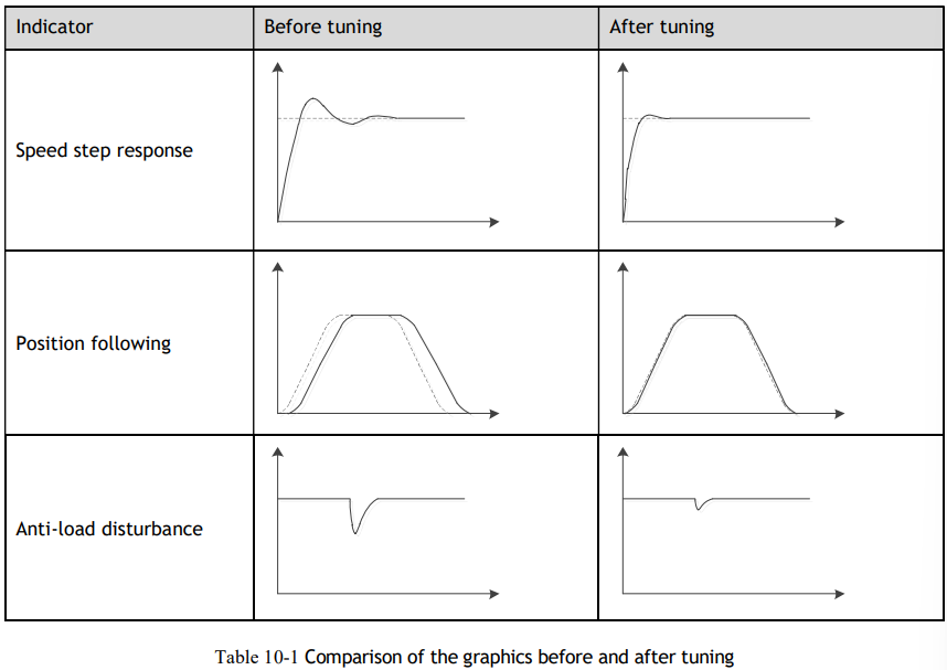
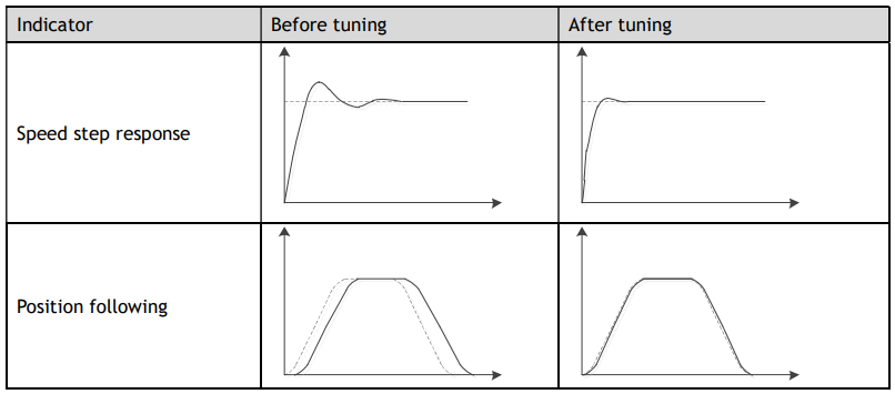
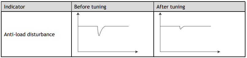
In general, the indicators used to evaluate Servo performance are bandwidth, response time, overshoot, steady state error, anti-load disturbance, speed ripple fluctuation, torque ripple, and so on. Table 10-1 shows the comparison of the graphics before and after tuning in the example indicators. 

10.1.2 Control Block Diagram
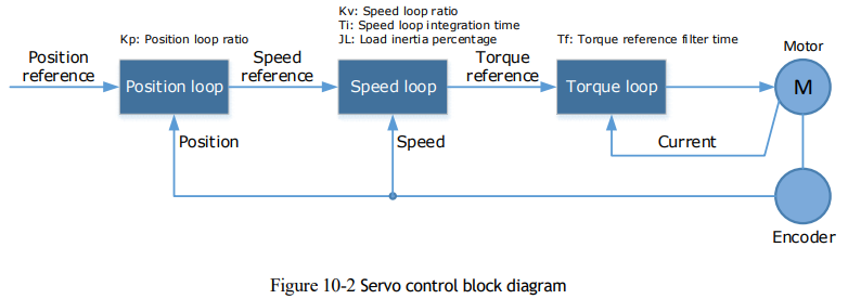
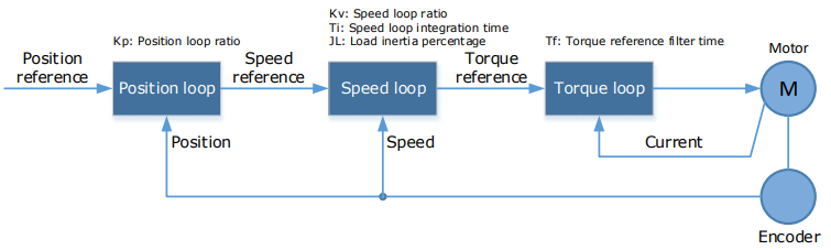
It is necessary to learn the Servo control principle and Figure 10-2 shows the Servo control block diagram.
The position loop, the speed loop and the torque loop are cascade structures, corresponding to the position control mode, the speed control mode, and the torque control mode, respectively. 

10.1.3 Tuning Process
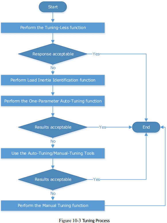
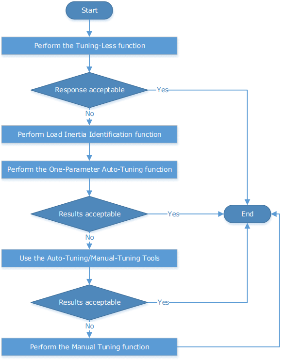
The Drive provides a variety of tuning methods, you can adjust the device according to the process shown in Figure 10-3, in order to obtain the desired Servo performance. 

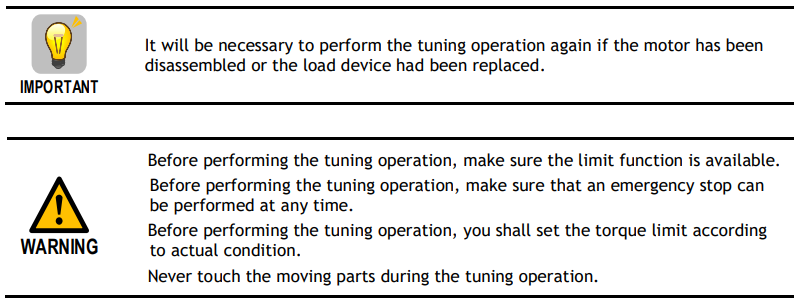
10.1.4 Precautions Before Tuning 

10.2 Tuning Modes
Tuning is the process of satisfying the servo performance by adjusting the parameters involved in the control law.
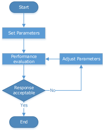
The process of tuning is usually an iterative process; the figure below shows the general flow.

There are various indicators used to evaluate servo performance including bandwidth, response time, overshoot, steady state error, anti-load disturbance, speed ripple fluctuation, torque ripple, etc. The importance of these will depending on the application.
The table below shows examples of speed vs time graphs showing the comparison of before and after tuning. 

10.3 Tuning Process
When tuning a servo drive is if helpful to understand the servo control principle used. The figure below shows the servo control block diagram. The position loop, the speed loop and the torque loop are cascaded structures, corresponding to the position control mode, the speed control mode, and the torque control mode, respectively. 

For tuning the drive follow the process below. 

10.4 Tuning Modes
The drive supports 3 different tuning modes, and different features are available in each mode.
Tuning-less: the drive performs auto-tuning to obtain a stable response regardless of the type of machine or changes in the load.
One-Parameter Auto-Tuning: similar to the tuning-less function but requires an inertia measurement of the load and uses a rigidity parameter to control the system bandwidth.
Manual Tuning: all gain terms are manually adjusted.
The tuning mode can be changed from the Tuning page in the drive commissioning screens. Click on the ‘Change Tuning Mode’ button. 

This will launch a wizard to guide the change of tuning mode.
Alternatively, the tuning mode can be changed by directly writing to parameter Pn100.0.

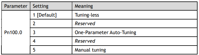
Once the tuning mode has been changed the drive will require a re-start for the new selection to apply.
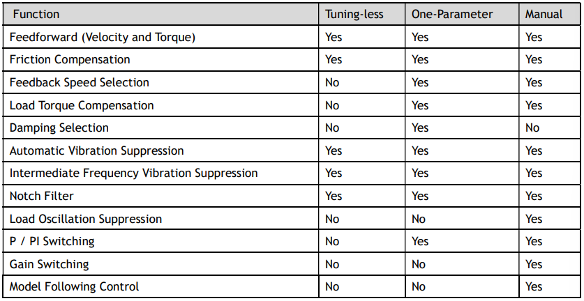
The table below show a summary functions available in each mode:

10.4.1 Tuningless
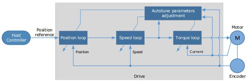
In Tuning-less mode the drive performs auto-tuning to obtain a stable response regardless of the type of machine or changes in the load. Autotuning is started when the servo is turned on.
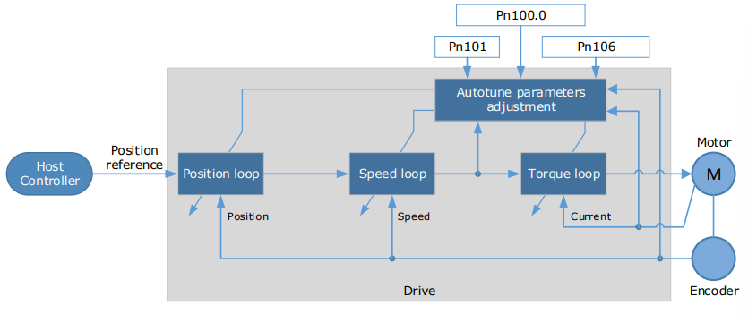
The tuning-less function uses an Autotune parameters adjustment module that updates the position loop and speed loop parameters in real time based on the servo operating state (position, speed, current). The figure below shows the block diagram in tuning-less.

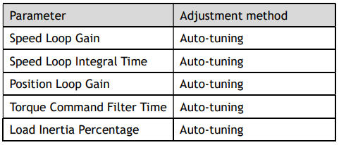
When using the tuning-less function, the following parameters are automatically adjusted. 

Use Case
Applicable for applications where the motor / load inertia mismatch is no more than 30 times.
Applicable for applications of any motor speed.

Parameters 

Changing the tuning mode will require the drive to be restarted.

Restrictions
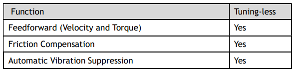
The following table shows a summary of functions available in tuning-less mode. 

10.4.2 One-Parameter Auto Tuning
This tuning function is similar to the tuning-less function, using an Autotune parameters adjustment module that updates the position loop and speed loop parameters in real time based on the servo operating state (position, speed, current).
One-Parameter Auto Tuning may offer some advantages over Tuning-less mode due to:
 Tuning is based on a proper load inertia percentage so tends to offer improved performance.
 The user selection of rigidity means that the tuning mode can be applied to more operating conditions.

One-Parameter Auto Tuning requires an inertia measurement of the load. The drive can measure the load inertia using the Inertia Detection tool, which can be launched from the Tuning page in the drive commissioning screens.

This will launch a wizard to guide the process of inertia detection.
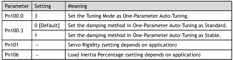
Alternatively, the inertia can be entered by directly writing to parameter Pn106.

The stiffness of the control is selected by a rigidity parameter. This can be adjusted by a slider on the
Tuning page in the drive commissioning screens.

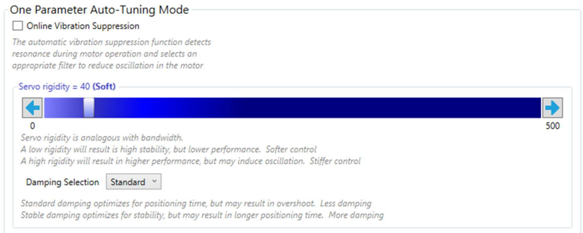
Alternatively, the rigidity can be entered by directly writing to parameter Pn101.

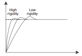
A lower number corresponds to a lower rigidity, less stiff. This will provide a slower response.
A higher number corresponds to a higher rigidity, stiffer. This will provide a faster response but taken too far may result in oscillation.

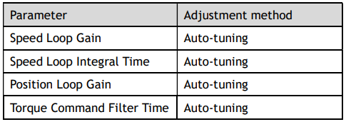
When using the One-Parameter Auto-Tuning function, the following parameters are automatically adjusted.

Use Case
Applicable for applications where the motor / load inertia mismatch is no more than 50 times.
Applicable for applications of any motor speed. 

Parameters 

Changing the tuning mode will require the drive to be restarted.

Restrictions
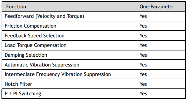
The following table shows a summary of functions available in one-parameter auto-tuning mode. 

10.4.3 Manual Tuning
In the Manual Tuning, the gain parameters are manually adjusted without using the autotune parameter adjustment module, until the desired performance is achieved. 

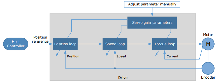
It is necessary to adjust the three-loop control parameters of the Servo from the inside out, that is, the adjustment sequence is Torque loop → Speed loop → Position loop. In order to maintain stability, the bandwidth setting should be the largest in the torque loop, then the speed loop, and the position loop should be smallest.
The following parameters need to be adjusted in each loop when performing Manual Tuning. 

Torque loop (Torque Control Mode)
 Torque Reference Filter Time (Tf):
The torque reference filter applies to the torque reference to remove the high frequency components, which can effectively reduce the torque ripple of the motor output, eliminate signal noise and reduce the temperature rise of the motor.
The larger the Torque Reference Filter Time, the better the filtering effect on the torque reference.
However, the greater the phase lag, and the slower the torque response. Therefore, the smallest acceptable value should be set to obtain a larger torque loop bandwidth in the actual tuning.
Speed loop (Speed Control Mode)
 Relevant parameter in torque loop (Tf)
 Load Inertia Percentage (JL)
Properly setting the Load Inertia Percentage is a prerequisite for the tuning to obtain the best performance. This can be calculated manually or measured using the Inertia Detection tool which is accessible from the Tuning page in the drive commissioning screens.
 Speed Loop Gain (Kv), Speed Loop Integral Time (Ti)
The speed loop is controlled using a Proportional-Integral Controller that contains Speed Loop Gain and Speed Loop Integral Time. Both determine the speed loop bandwidth and anti-disturbance performance of the Servo.
In general, increasing the setting of the Speed Loop Gain will increase the speed loop bandwidth, and the anti-load disturbance performance will be better. Decreasing the setting of the Speed Loop Integral Time will strengthen the integral action, the speed loop bandwidth will be increased, and the anti-load disturbance performance will be better. In addition, the integral action may reduce the steady-state error to zero.
The table below lists several commonly used adjustment methods based on the characteristics of the speed step response. 

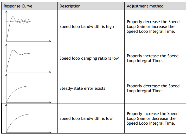
It is recommended to increase the Speed Loop Gain and decrease the Speed Loop Integral Time to obtain a larger speed loop bandwidth.
Position loop (Position Control Mode)
 Relevant parameters in speed loop (Kv, Ti, Tf, and JL)
 Position Loop Gain (Kp)
The position loop is controlled using a Proportional Controller that only contains the Position Loop Gain. This parameter determines the position loop bandwidth. Increasing the Position Loop Gain will increase the position loop bandwidth, and the anti-load disturbance performance will be better. If the Position Loop Gain is too high this will cause overshooting and vibration.
It is recommended to set the Position Loop Gain to a quarter of the Speed Loop Gain, and make appropriate adjustments based on this.
Access to all control law parameters is available from the Tuning page or the Parameter page in the drive commissioning screens.
Use Case
Applicable for applications where the motor / load inertia mismatch is no more than 50 times.
Applicable for applications of any motor speed.

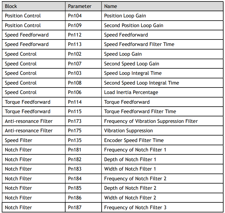
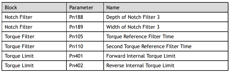
The parameters for manual tuning are:

Restrictions
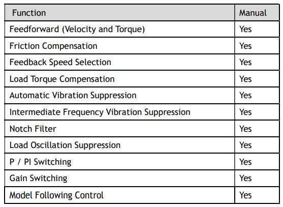
The following table shows a summary of functions available in manual tuning mode

10.5 Compensation
The Drive offers several compensation techniques which can be used in various tuning modes to improve performance.
10.5.1 Feedforward
The table below shows the tuning modes where the feed forward function can be used. 

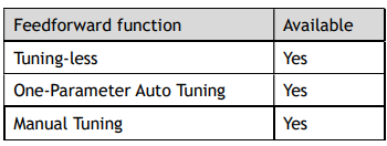
Feedforward includes both speed feedforward and torque feedforward.
 Speed feedforward can improve position response and reduce position following error.
 Torque feedforward can improve the speed response and reduce the speed following error.

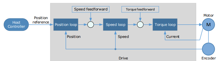
In general, the differential of the position reference is used as the feedforward. This is known as an internal feedforward reference and is the default mode of operation. Other options are available for generating the feedforward reference.
 Internal Feedforward (default)
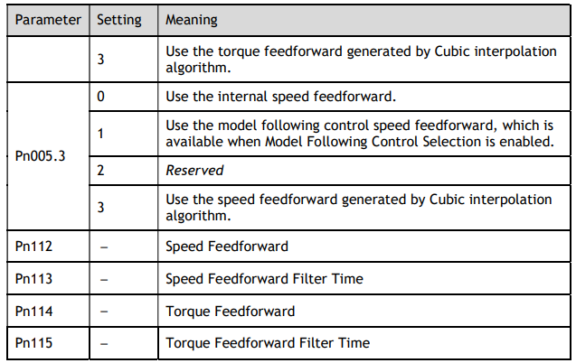
 Model Following Feedforward, available when Model Following Control is selected.
 Cubic feedforward
Internal Feedforward
When using internal feedforward the reference is calculated using:
 Internal Speed Feedforward ＝
Differential of position reference × Speed Feedforward
 Internal Torque Feedforward ＝
Differential of speed reference × Load Inertia Percentage × Torque Feedforward
 Increasing the feedforward term will tend to reduce error during periods where the reference is constant. i.e. during periods of constant speed, the speed feed forward will allow to the control scheme to reduce following error, however the feedforward can introduce overshoot.
In addition, it may be required to filter the noise caused by the differential for the feedforward.
Increasing the filter time will reduce the noise but may increase the overshoot.
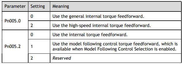
In the case of high rotation speed, it may be necessary to use the high-speed torque feed forward function, this is selected by setting parameters:
 Pn005.0 to 2 (select high-speed internal torque feedforward)
 Pn005.2 to 0 (use internal torque feedforward)
Model Following Control Feedforward
This is only available when the Model Following Control function has been enabled.
For details on this method, refer to the section 10.8 Model Control Following.
Cubic Interpolation
Uses a cubic algorithm for interpolation of the reference.
Parameters