10. Tuning

10.1 Overview
10.1.1 Basic Conception
Tuning is the process of satisfying the servo performance by adjusting the parameters involved in the
control law.

Tuning Flow
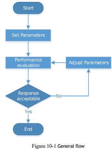
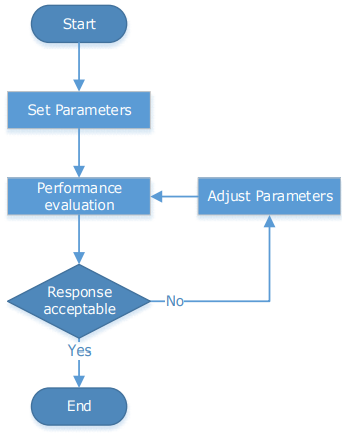
The process of tuning is usually an iterative process, and Figure 10-1 shows the general flow.

Parameter Classification
There are two types of parameters in the tuning.
 Function Parameters: refers to some application function selections or switches that may improve Servo performance.
 Adjustment Parameters: increasing or decreasing these parameters may improve Servo performance.

Servo Performance
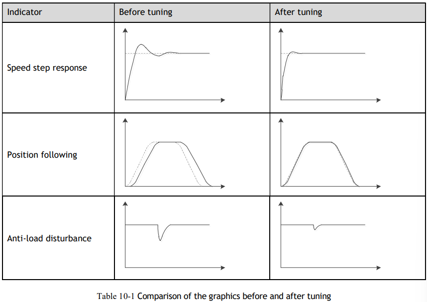
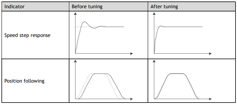
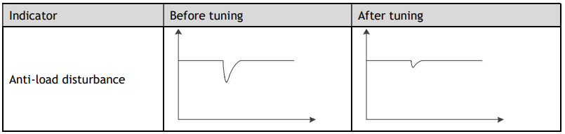
In general, the indicators used to evaluate Servo performance are bandwidth, response time, overshoot, steady state error, anti-load disturbance, speed ripple fluctuation, torque ripple, and so on. Table 10-1 shows the comparison of the graphics before and after tuning in the example indicators.

10.1.2 Control Block Diagram
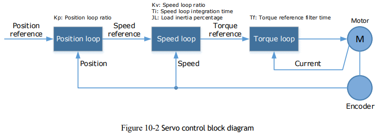
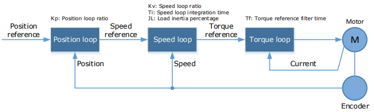
It is necessary to learn the Servo control principle and Figure 10-2 shows the Servo control block diagram.
The position loop, the speed loop and the torque loop are cascade structures, corresponding to the position control mode, the speed control mode, and the torque control mode, respectively.

10.1.3 Tuning Process
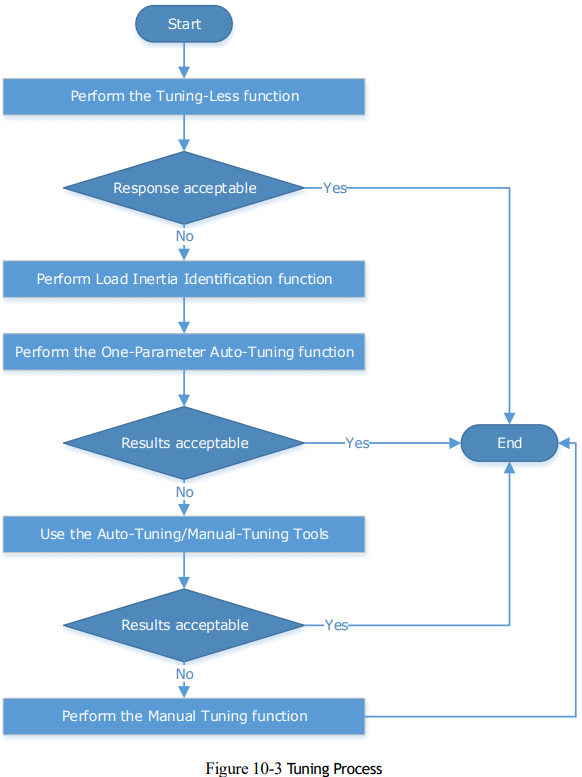
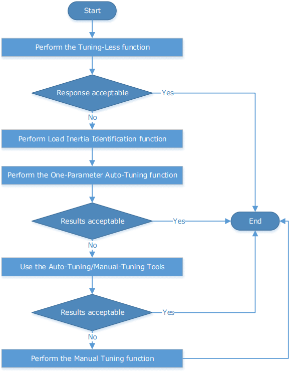
The Drive provides a variety of tuning methods, you can adjust the device according to the process shown in Figure 10-3, in order to obtain the desired Servo performance.

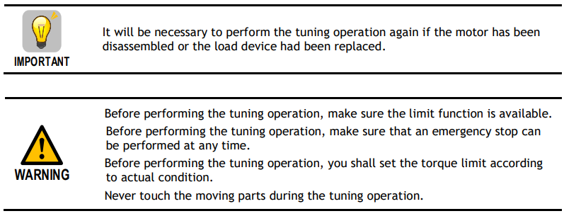
10.1.4 Precautions Before Tuning

10.2 Tuning Modes
Tuning is the process of satisfying the servo performance by adjusting the parameters involved in the control law.
The process of tuning is usually an iterative process; the figure below shows the general flow.

There are various indicators used to evaluate servo performance including bandwidth, response time, overshoot, steady state error, anti-load disturbance, speed ripple fluctuation, torque ripple, etc. The importance of these will depending on the application.
The table below shows examples of speed vs time graphs showing the comparison of before and after tuning.

10.3 Tuning Process
When tuning a servo drive is if helpful to understand the servo control principle used. The figure below shows the servo control block diagram. The position loop, the speed loop and the torque loop are cascaded structures, corresponding to the position control mode, the speed control mode, and the torque control mode, respectively.

For tuning the drive follow the process below.

10.4 Tuning Modes
The drive supports 3 different tuning modes, and different features are available in each mode.
Tuning-less: the drive performs auto-tuning to obtain a stable response regardless of the type of machine or changes in the load.
One-Parameter Auto-Tuning: similar to the tuning-less function but requires an inertia measurement of the load and uses a rigidity parameter to control the system bandwidth.
Manual Tuning: all gain terms are manually adjusted.
The tuning mode can be changed from the Tuning page in the drive commissioning screens. Click on the ‘Change Tuning Mode’ button.

This will launch a wizard to guide the change of tuning mode.
Alternatively, the tuning mode can be changed by directly writing to parameter Pn100.0.

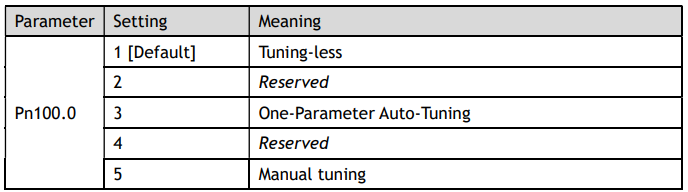
Once the tuning mode has been changed the drive will require a re-start for the new selection to apply.
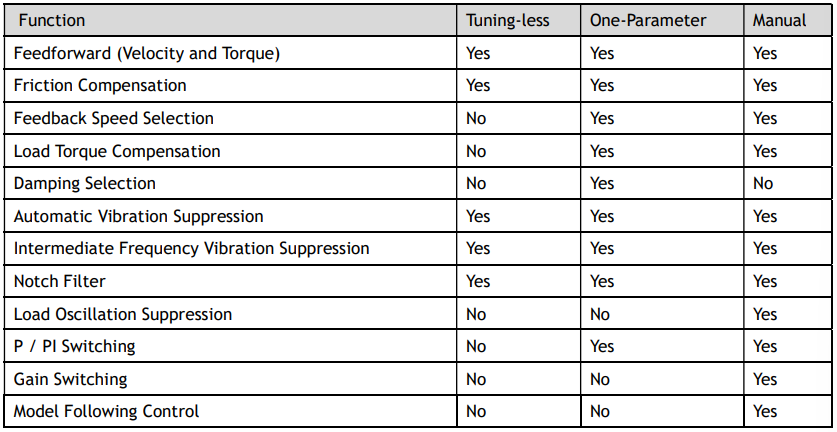
The table below show a summary functions available in each mode:

10.4.1 Tuningless
In Tuning-less mode the drive performs auto-tuning to obtain a stable response regardless of the type of machine or changes in the load. Autotuning is started when the servo is turned on.
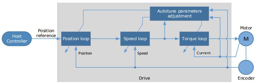
The tuning-less function uses an Autotune parameters adjustment module that updates the position loop and speed loop parameters in real time based on the servo operating state (position, speed, current). The figure below shows the block diagram in tuning-less.

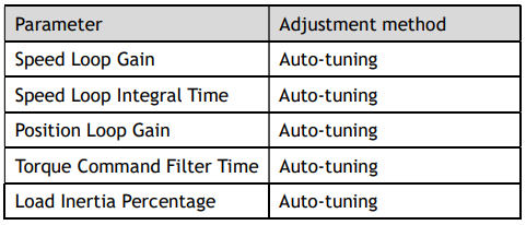
When using the tuning-less function, the following parameters are automatically adjusted.

Use Case
Applicable for applications where the motor / load inertia mismatch is no more than 30 times.
Applicable for applications of any motor speed.

Parameters

Changing the tuning mode will require the drive to be restarted.

Restrictions
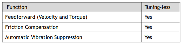
The following table shows a summary of functions available in tuning-less mode.

10.4.2 One-Parameter Auto Tuning
This tuning function is similar to the tuning-less function, using an Autotune parameters adjustment module that updates the position loop and speed loop parameters in real time based on the servo operating state (position, speed, current).
One-Parameter Auto Tuning may offer some advantages over Tuning-less mode due to:
 Tuning is based on a proper load inertia percentage so tends to offer improved performance.
 The user selection of rigidity means that the tuning mode can be applied to more operating conditions.

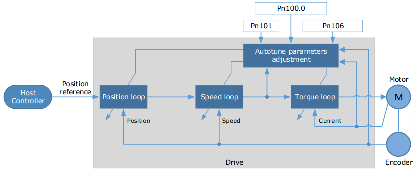
One-Parameter Auto Tuning requires an inertia measurement of the load. The drive can measure the load inertia using the Inertia Detection tool, which can be launched from the Tuning page in the drive commissioning screens.

This will launch a wizard to guide the process of inertia detection.
Alternatively, the inertia can be entered by directly writing to parameter Pn106.

The stiffness of the control is selected by a rigidity parameter. This can be adjusted by a slider on the
Tuning page in the drive commissioning screens.

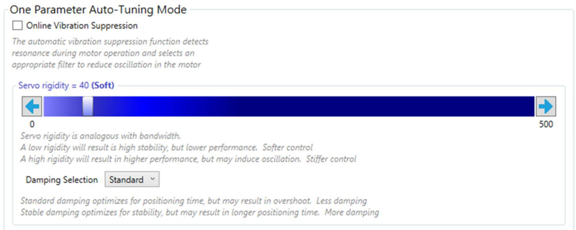
Alternatively, the rigidity can be entered by directly writing to parameter Pn101.

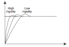
A lower number corresponds to a lower rigidity, less stiff. This will provide a slower response.
A higher number corresponds to a higher rigidity, stiffer. This will provide a faster response but taken too far may result in oscillation.

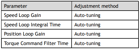
When using the One-Parameter Auto-Tuning function, the following parameters are automatically adjusted.

Use Case
Applicable for applications where the motor / load inertia mismatch is no more than 50 times.
Applicable for applications of any motor speed.

Parameters

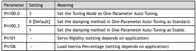
Changing the tuning mode will require the drive to be restarted.

Restrictions
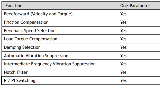
The following table shows a summary of functions available in one-parameter auto-tuning mode.

10.4.3 Manual Tuning
In the Manual Tuning, the gain parameters are manually adjusted without using the autotune parameter adjustment module, until the desired performance is achieved.

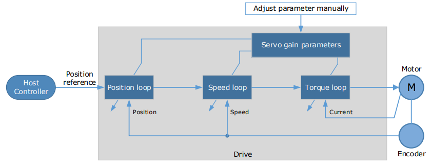
It is necessary to adjust the three-loop control parameters of the Servo from the inside out, that is, the adjustment sequence is Torque loop → Speed loop → Position loop. In order to maintain stability, the bandwidth setting should be the largest in the torque loop, then the speed loop, and the position loop should be smallest.
The following parameters need to be adjusted in each loop when performing Manual Tuning.

Torque loop (Torque Control Mode)
 Torque Reference Filter Time (Tf):
The torque reference filter applies to the torque reference to remove the high frequency components, which can effectively reduce the torque ripple of the motor output, eliminate signal noise and reduce the temperature rise of the motor.
The larger the Torque Reference Filter Time, the better the filtering effect on the torque reference.
However, the greater the phase lag, and the slower the torque response. Therefore, the smallest acceptable value should be set to obtain a larger torque loop bandwidth in the actual tuning.
Speed loop (Speed Control Mode)
 Relevant parameter in torque loop (Tf)
 Load Inertia Percentage (JL)
Properly setting the Load Inertia Percentage is a prerequisite for the tuning to obtain the best performance. This can be calculated manually or measured using the Inertia Detection tool which is accessible from the Tuning page in the drive commissioning screens.
 Speed Loop Gain (Kv), Speed Loop Integral Time (Ti)
The speed loop is controlled using a Proportional-Integral Controller that contains Speed Loop Gain and Speed Loop Integral Time. Both determine the speed loop bandwidth and anti-disturbance performance of the Servo.
In general, increasing the setting of the Speed Loop Gain will increase the speed loop bandwidth, and the anti-load disturbance performance will be better. Decreasing the setting of the Speed Loop Integral Time will strengthen the integral action, the speed loop bandwidth will be increased, and the anti-load disturbance performance will be better. In addition, the integral action may reduce the steady-state error to zero.
The table below lists several commonly used adjustment methods based on the characteristics of the speed step response.

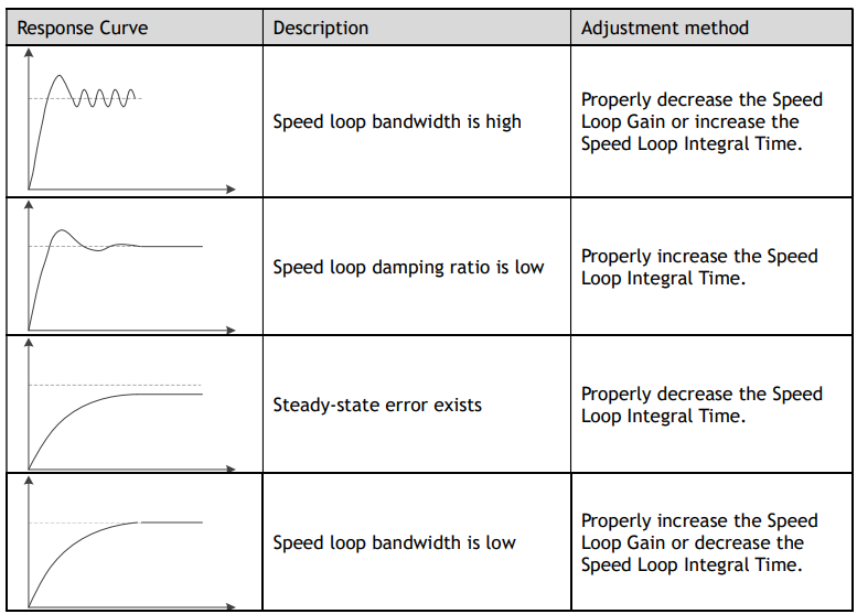
It is recommended to increase the Speed Loop Gain and decrease the Speed Loop Integral Time to obtain a larger speed loop bandwidth.
Position loop (Position Control Mode)
 Relevant parameters in speed loop (Kv, Ti, Tf, and JL)
 Position Loop Gain (Kp)
The position loop is controlled using a Proportional Controller that only contains the Position Loop Gain. This parameter determines the position loop bandwidth. Increasing the Position Loop Gain will increase the position loop bandwidth, and the anti-load disturbance performance will be better. If the Position Loop Gain is too high this will cause overshooting and vibration.
It is recommended to set the Position Loop Gain to a quarter of the Speed Loop Gain, and make appropriate adjustments based on this.
Access to all control law parameters is available from the Tuning page or the Parameter page in the drive commissioning screens.
Use Case
Applicable for applications where the motor / load inertia mismatch is no more than 50 times.
Applicable for applications of any motor speed.

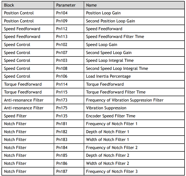
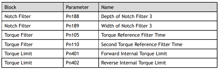
The parameters for manual tuning are:

Restrictions
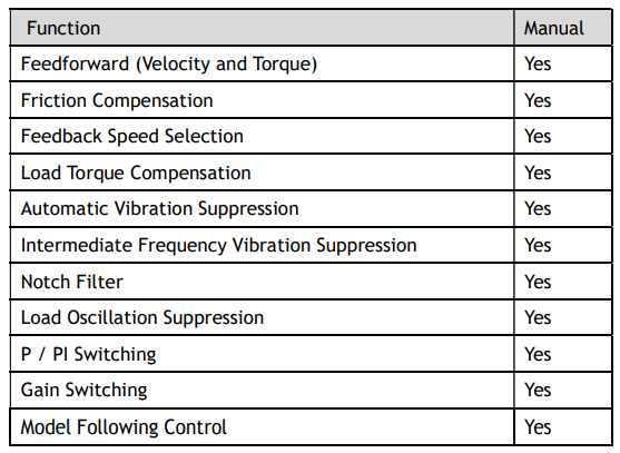
The following table shows a summary of functions available in manual tuning mode

10.5 Compensation
The Drive offers several compensation techniques which can be used in various tuning modes to improve performance.
10.5.1 Feedforward
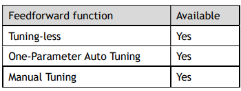
The table below shows the tuning modes where the feed forward function can be used.

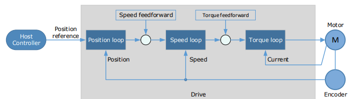
Feedforward includes both speed feedforward and torque feedforward.
 Speed feedforward can improve position response and reduce position following error.
 Torque feedforward can improve the speed response and reduce the speed following error.

In general, the differential of the position reference is used as the feedforward. This is known as an internal feedforward reference and is the default mode of operation. Other options are available for generating the feedforward reference.
 Internal Feedforward (default)
 Model Following Feedforward, available when Model Following Control is selected.
 Cubic feedforward
Internal Feedforward
When using internal feedforward the reference is calculated using:
 Internal Speed Feedforward ＝
Differential of position reference × Speed Feedforward
 Internal Torque Feedforward ＝
Differential of speed reference × Load Inertia Percentage × Torque Feedforward
 Increasing the feedforward term will tend to reduce error during periods where the reference is constant. i.e. during periods of constant speed, the speed feed forward will allow to the control scheme to reduce following error, however the feedforward can introduce overshoot.
In addition, it may be required to filter the noise caused by the differential for the feedforward.
Increasing the filter time will reduce the noise but may increase the overshoot.
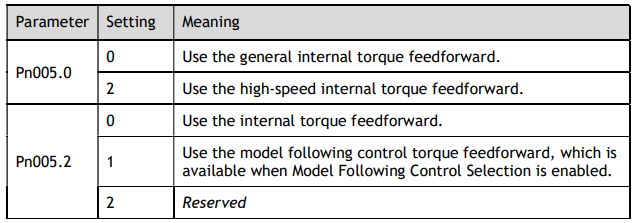
In the case of high rotation speed, it may be necessary to use the high-speed torque feed forward function, this is selected by setting parameters:
 Pn005.0 to 2 (select high-speed internal torque feedforward)
 Pn005.2 to 0 (use internal torque feedforward)
Model Following Control Feedforward
This is only available when the Model Following Control function has been enabled.
For details on this method, refer to the section 10.8 Model Control Following.
Cubic Interpolation
Uses a cubic algorithm for interpolation of the reference.
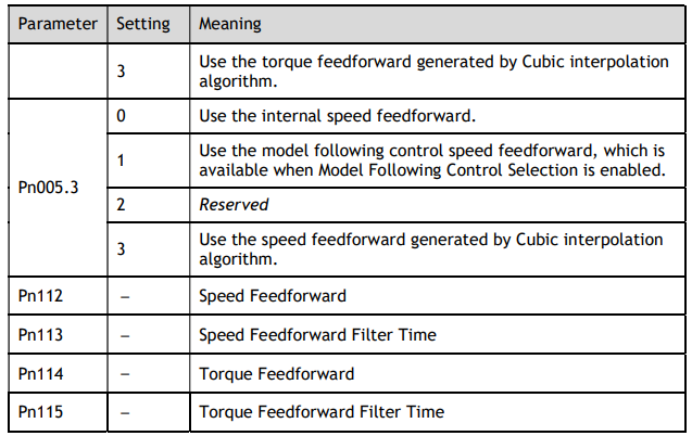
Parameters

10.5.2 Friction Compensation
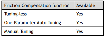
The table below shows the tuning modes where the friction compensation function can be used.

Load friction will exist in the transmission system. However, severe load friction may cause low-speed crawling, waveform distortion at speed zero-crossing, positioning lag, etc. This can affect the dynamic and static performance of the system. The friction compensation function allows the drive to compensate for this and may be a requirement in applications with frequent forward and reverse motion, and high speed-stability requirements.
Friction compensation is used to compensate for both viscous friction fluctuations and coulomb friction fluctuations.
Coulomb Friction Compensation
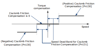
Coulomb friction compensation is controlled though parameters Pn130 and Pn131.

The application of coulomb friction compensation is symmetrical around zero speed. It is advisable to set a dead band for the friction compensation to avoid the system changing the compensation direction frequently near zero speed.
The diagram below shows the application of coulomb friction compensation.

Viscous friction compensation is controlled though parameter Pn132

The application of viscous friction compensation is a linear relationship with the actual speed, as is shown below.

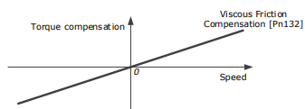
As the speed increase, so the viscous friction compensation increases with a rate defined by the Viscous Friction Compensation parameter.

10.5.3 Speed Feedback Selection
The table below shows the tuning modes where the speed feedback function can be used.

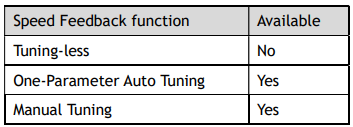
By default, the speed feedback is calculated from by differentiating the positional value read from the encoder.
In the case of low speed or low encoder resolution, the method of position differentiation to calculate speed can introduce a large amount of noise in speed feedback which can affect the control performance.
To reduce the noise, a low pass filter can be applied to eliminate the noise and high-frequency components from the speed signal. The speed filter is controller though the Encoder Speed Filter Time parameter.

Increase the time constant of the filter will have a stronger effect on the noise resulting in a smoother speed signal. But a strong filter will introduce phase lag, which can reduce the servo performance.

An alternative to using encoder position to calculate speed is to use a speed observer, this can provide a less noisy speed. The observed speed can be tuned to match actual speed using the Load Torque Observer Gain; however, this may introduce overshoot.

10.5.4 Load Torque Compensation
The table below shows the tuning modes where the load torque compensation function can be used.

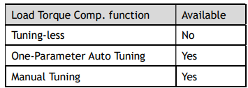
Sudden changes in load torque can significantly affect the speed control during operation. A step change in load torque will introduce a decrease in speed which will take some time for the control to rectify.
In applications with continuously changing load torque, it is necessary to improve the anti-load disturbance performance of the servo.
The figure below shows the speed drop caused by a sudden load torque. The load torque compensation function can be used to reduce the effect of the load torque change.

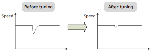
Tuning the load torque compensation function can be used to improve the anti-load disturbance performance, considering that the reference response performance and the load disturbance resistance cannot be balanced.
The Load Torque Compensation function adjusts compensation to the torque reference via an observer function. To reduce the overshoot caused by Load Torque Compensation, use the load torque compensation percentage to adjust the compensation value:
Load Torque Compensation ＝ Load Torque Observer × Load Torque Compensation Percentage

Increasing this value can improve the load disturbance rejection performance. Too much may cause vibration and overshoot.
In addition, the bandwidth of the load torque observer can be changed via Load Torque Observer Gain.
Increasing this will make the observed torque closer to the actual torque but may generate overshoot.

10.5.5 Damping Selection
The table below shows the tuning modes where the damping selection function can be used.

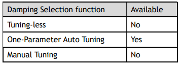
The Damping Selection selects between 2 damping options.
 [0] Standard: Short positioning time, but prone to overshoot.
 [1] Stable: Longer positioning time, but stable.

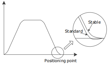
The damping selection can be made from the Tuning page in the drive commissioning screens.
Alternatively, the damping selection can be changed by directly writing to parameter Pn100.3.

10.6 Vibration Suppression
The Drive offers several vibration suppression techniques which can be used in various tuning modes to improve performance.

10.6.1 Automatic Vibration Suppression
The table below shows the tuning modes where the automatic vibration suppression function can be used.

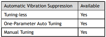
The automatic vibration suppression function determines the vibration state of the Motor during operation and identifies the resonant frequency. It then selects either the Notch Filter or the IF Vibration

Suppression according to the characteristics of the vibration. It will set the parameters for IF Vibration Suppression or Notch Filter 2, depending on what is required.
Automatic Vibration Suppression can be enabled from the Tuning screen in the drive parameter pages.
Alternatively, the this can be controlled by directly writing to parameter Pn100.2.

To prevent the automatic vibration suppression acting on incorrect vibrations an amplitude threshold can be applied can. This will prevent the vibration suppression acting on any detected frequency unless it exceeds the threshold.

10.6.2 IF (Intermediate Frequency) Vibration Suppression
The table below shows the tuning modes where the IF vibration suppression function can be used

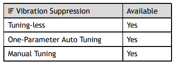
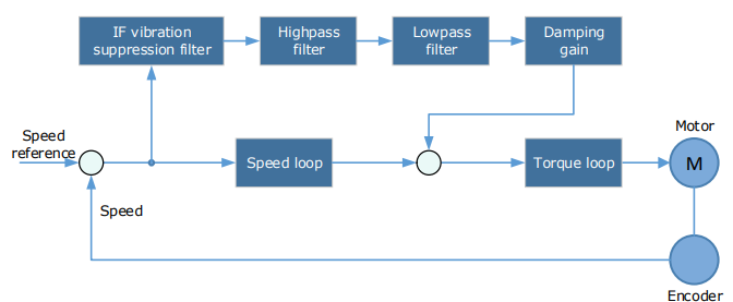
The IF vibration suppression filter is used to process the speed deviation and provide compensation to the torque reference. It is applied for the frequency range 100 Hz to 2000 Hz.

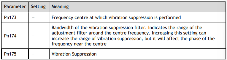
NOTE: Set Pn173 to 2000, indicating the notch filter is unavailable

10.6.3 Notch Filter
The table below shows the tuning modes where the notch filter function can be used.

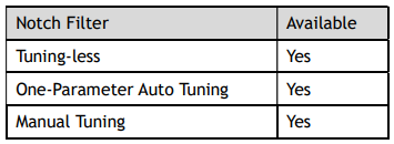
The notch filter is used to eliminate vibration caused by mechanical resonance.
There are three notch filters in the Drive, those who can used independently or in combination.

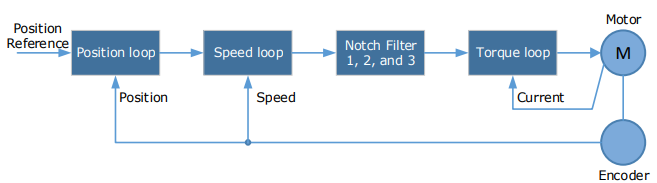
The diagram below shows the relevant parameters for the notch filter.
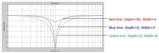
Notch filter can attenuate the signal at a specific frequency so can be very useful in removing resonance. Setting a correct frequency and width the vibration signal in the torque reference can be filtered out.

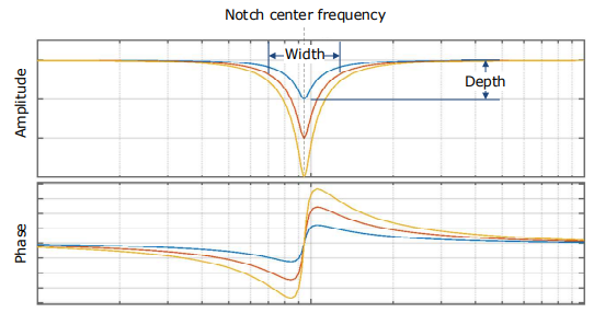
Parameters controlling the operation of notch filter are:
 Frequency, setting the frequency of notch filter to 5000 will disable the notch filter.
 Depth, the range of depth is from 0 to 23.
 Width, the range of width is from 0 to 15.

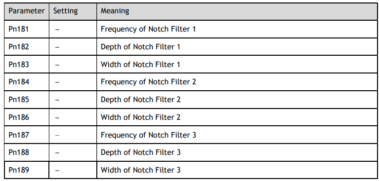
The notch filter parameters can be set from the Tuning page in the drive commissioning screens.
Alternatively, the filters can be configured by directly writing to the parameters.

10.6.4 Load Oscillation Suppression
The table below shows the tuning modes where the load oscillation suppression function can be used.

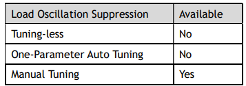
The Load Oscillation Suppression function is used for suppressing low frequency jitter at the end of the load during position control.

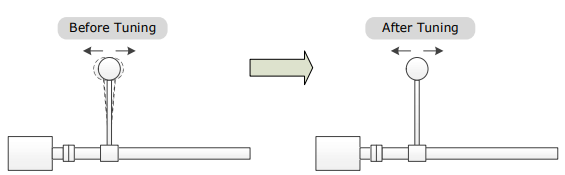
The aim of the Model Following Control is to maintain the stability of the load position based on a relationship between load position and Motor position. This is done by correcting the position reference and generating new speed and torque feedforward values.
The block diagram below shows Load Oscillation Suppression.

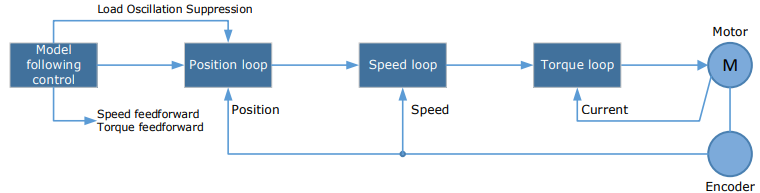
This function is based on the Model Following Control (10.8 ) and enabled via Pn150.

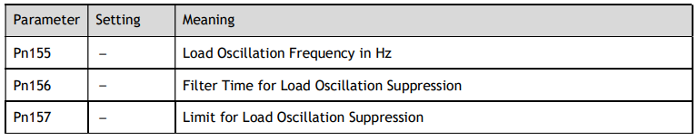
Parameters controlling the operation of load oscillation suppression are:
 Frequency, which specifies the frequency at which Load Oscillation Suppression is to be performed.
 Filter Time, increasing this setting will strengthen the filter. However, it may reduce the suppression effect due to lag.
 Limit, which will clip the output of the Load Oscillation Suppression, helping to reduce overshooting during starting and stopping.

10.7 Gain Scheduling
The Drive offers several gain scheduling techniques which can be used in various tuning modes to improve performance.

10.7.1 P/PI Switching
The table below shows the tuning modes where the P/PI switching function can be used

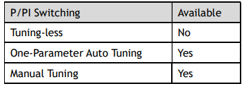
By default, the Drive uses a Proportional-Integral (PI) Controller for the speed loop. This can be changed from PI to P control based on some reference condition using parameter Pn116.

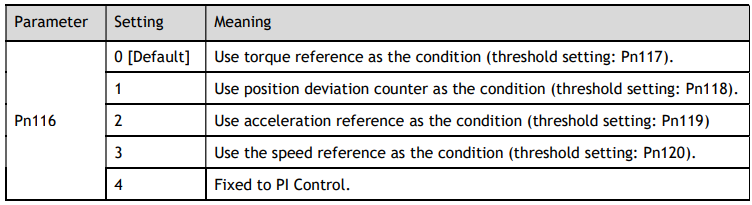
The relevant threshold parameters are shown in the table below.

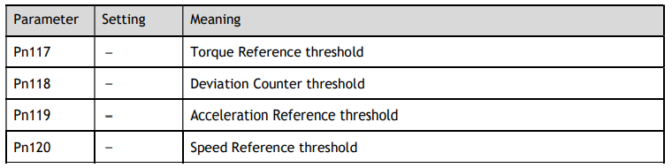
Consider the default settings as an example. The default setting is to use torque reference as the condition, and the default Torque Reference threshold (Pn117) is 200.
 When the torque reference percentage is less than 200, the speed loop adjustment will be PI control.
 When the torque reference percentage is greater than 200, the speed loop adjustment will be P
control.

10.7.2 Gain Switching
The table below shows the tuning modes where the gain switching function can be used.

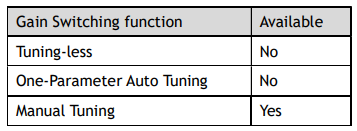
In manual tuning mode a gain switching function can be used which allows the drive to swap between two sets of gain parameters based on operating conditions.

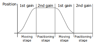
The figure below shows an example:
 The ‘positioning’ gain terms focus on the performance such as position ripples and positional rigidity
 The ‘moving’ gain terms focus on the performance such as following error.
In this case, two switchable groups of gain parameters are required to meet the servo performance.

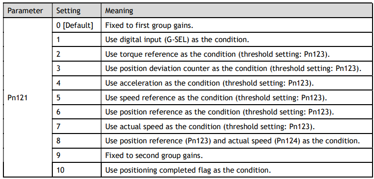
Gain switching can be enabled from the Tuning page in the drive commissioning screens. The conditions for gain switching are selected from a drop down.
Options are:
 Fixed to first group gains.
 Use digital input (G-SEL) as the condition.
 Use torque reference as the condition.
 Use position deviation counter as the condition.
 Use acceleration as the condition.
 Use speed reference as the condition.
 Use position reference as the condition.
 Use actual speed as the condition.
 Use position reference and actual speed as the condition.
 Fixed to second group gains.
 Use positioning completed flag as the condition.
Once gain switching is selected the switch conditions will be shown.

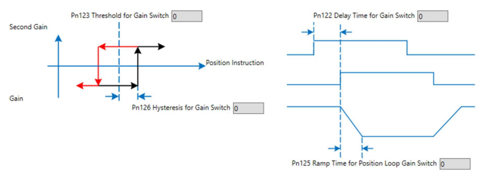
And any additional gain terms parameters will be available from the control law block diagram

Alternatively, gain switching can be enabled by directly to the parameters.

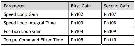
The parameters for the first gain and the second gain terms are as follows.

10.8 Model Control Following
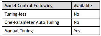
The table below shows the tuning modes where the model control following function can be used.

The Model Following Control is a function which sits before the position loop. In Model Following Control, new position references are generated based on the theoretical Motor control model, and relevant speed feedforward and torque feedforward are generated.
Applying these controls to the actual control loop can significantly improve the response performance and positioning performance of the position control.
The block diagram below shows the implementation of model following control.

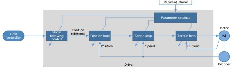
The Model Following Control function is enabled via Pn150.

To use the Model Following Control properly, the system should be setup in the following order:

For details on the relevant parameter of Torque Loop, Speed Loop and Position Loop, refers to the sectio 10.4.3 Manual Tuning.

The relevant parameters for Model Following Control are as follows.

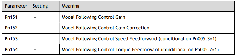
The gain determines the position response performance. Increasing this setting can improve speed of response, but overshooting is likely to occur.
The gain correction determines the damping ratio.
The (speed/torque) feedforward is a percentage factor that is used to adjust the feedforward value.

10.9 Load Identification
There are several tools which can be used help the tuning process.

10.9.1 Load Inertia Identification
The table below shows the tuning modes where the load inertia identification function can be used.

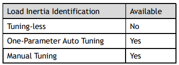
The Load Inertia Identification function is used to calculate the load inertia relative to the Motor rotor inertia (percentage of load inertia).
The Load Inertia Identification function can be started from the Tuning page in the drive commissioning screens. Click on the ‘Inertia Detection’ button.

This will launch a wizard to guide the inertia detection sequence.
The identification routine will rotate the Motor back and forth either 4 or 8 times, during this movement the inertia is calculated. At the end of the identification routine, the result is displayed with the option to update the inertia value in Pn106.
To perform this function the Drive must be disabled.

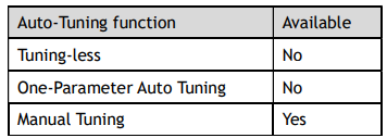
10.9.2 Auto-Tuning Tool
The table below shows the tuning modes where the auto tuning function can be used.

The Auto-Tuning Tool uses the drives internal position reference generator to exercise the Drive while iteratively changing the control parameters to achieve a tuned system.
The Auto-Tuning Tool can be started from the Tuning page in the drive commissioning screens. Click on the ‘Parameter Auto Tuning’ button.

This will launch a wizard to guide the parameter auto-tuning sequence.
The sequence is described in the flow chart below.

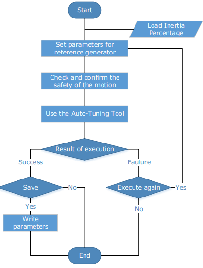
The steps in the wizard are:
 Detect Inertia
 Setup
 Motion Trajectory
 Tuning
 Results
Detect Inertia: A pre-request for the Parameter-Auto Tuning is an accurate measurement of inertia. This can be entered manually or measured using the Inertia Detection tool. For more details on inertia detection see 0There are several tools which can be used help the tuning process.
Load Inertia Identification.
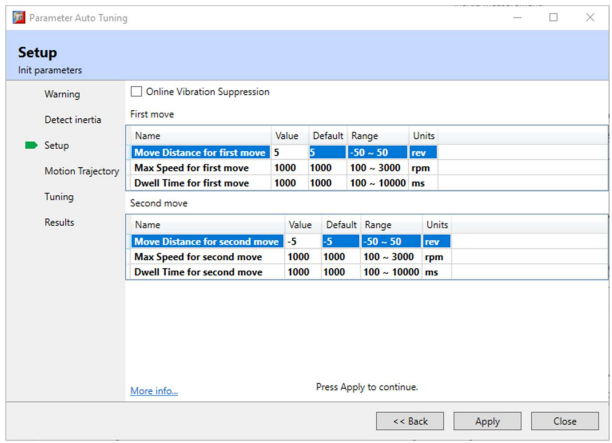
Setup: The drive will repeatedly run two moves during the Parameter Auto-Tuning, these are described by Distance, Speed and Dwell Time. The sequence can be either position/negative or negative/positive.

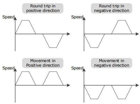
The Setup screen allows entry of the parameters which describe the motion

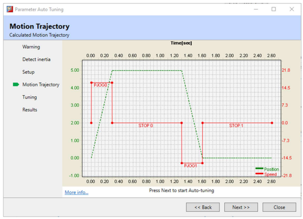
Motion Trajectory: This is an opportunity to review the defined motion sequence before starting the tuning sequence.

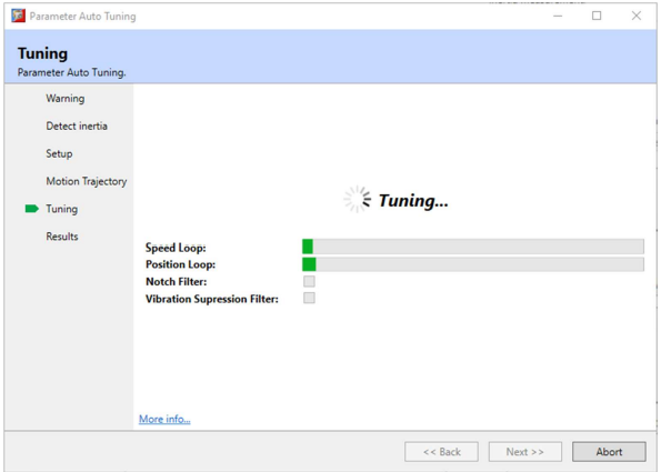
Tuning: During the internal tuning process, the progress is displayed on screen

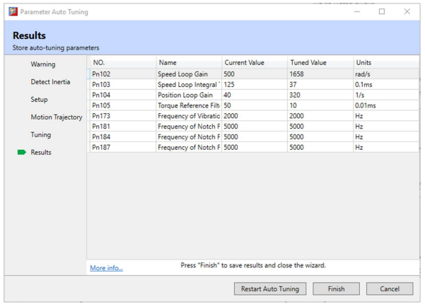
Results: Once the tuning process has completed, the calculated gain terms will be displayed with an option to save them to the drive.

10.10 Motor Overload Duration & Cycle Times

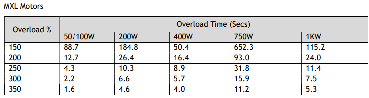
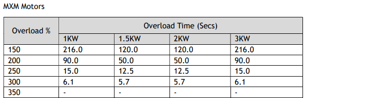
Care must be taken to ensure that the duty cycle is not exceeded when using high percentage overload durations.
For example:
Using a 400W motor at 350% the maximum time at this level must not exceed 4.0 secs.
The motor will now have to wait 45 secs before it is safe to run again at a higher level of percentag overload.
Off Time = (Overload % Factor^2 * Overload Time) - Overload Time
Off Time = (3.5 ² x 4.0) – 4.0 = 45.0s